Team:Edinburgh/Modeling/Whole cell model
From 2013.igem.org
Contents |
Whole cell model
Description
We chose to base our work on a whole cell model originally developed by Tobias Bollenbach (2009), tailored to capture the influence of different antibiotics on the growth rate and metabolism of E.coli. This model was suitable because it is a simple high-level model, and it was possible to understand and re-implement it within the time course of one summer. At the same time, it captures essential features of the cell metabolism which we might be interested in, such as resource availability, growth rate, and intracellular protein levels.
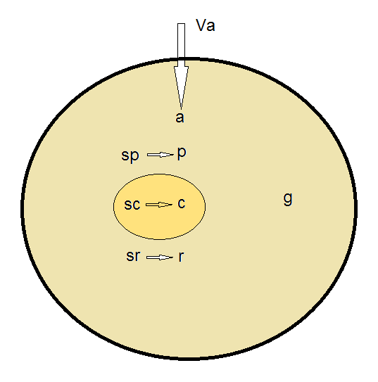
The model in the original paper assumes a constant influx of resources from the outer environment inside the cell. This resource influx is the only input to the model, and as a function of this resource level, the model can predict population average values for the following parameters (Figure 1):
- Growth rate
- Resource concentration inside the cell
- Protein number
- Amount of DNA
- Number of ribosomes
- Speeds of synthesis of proteins, ribosomes and DNA
- The cell volume
- Number of replication origins and forks in the cell
Figure 1. Simple diagram of the variables and relationships captured by the Bollenbach model
The model does not model RNA specifically, nor does it take into account the different proteins, their different expression levels and their different functions. Additionally, the model does not model degradation of proteins, only degradation of resources (which is supposed to capture resource usage by other factors which are not accounted for by the model).
The model constitutes a differential-algebraic system of equations, which track the evolution of the parameters over time. There are 4 differentiation equations and 11 algebraic equations, which respectively relate the instantaneous amount of resources, protein, ribosome and DNA to their synthetic rate, and describe the interactions (protein and ribosome synthesis, DNA replication etc.) in the cell at molecular level. Another equation is introduced to enable the system to achieve steady states, implicitly relating growth rate to protein synthesis rate. The predictions given by the model are found by finding the steady-state solution of the differential-algebraic system. This solution gives parameter averages which are expected to be found in the cell in a state of steady exponential growth.
The model makes the assumption that the ribosome synthesis rate is optimized for highest growth rate. Hence, the model runs an optimization algorithm over this parameter to find what is the best synthesis rate for the given resource influx rate before running the actual simulation for this resource environment.
Solving the system
We tried solving the system with different solvers from Mathematica and Matlab but we couldn’t get any of them to work. The reason is that the system of equations is quite complex, includes algebraic as well as differential equations and a lot of self-dependences between the variables. Some of the solvers didn’t allow for algebraic equations in the differential system, while others failed to solve the system altogether.
We decided to program our own solver based on time step integration. Firstly, we implemented the simplest possible model – Forward Euler – but we got a mathematical problem. For some levels of resource influx, the system never reached steady state, but kept oscillating between different sets of values for the parameters. Since the output of the system is the steady-state solution, the model didn’t give any predictions in these cases.
With help from Nicky from the SDU-Denmark iGEM team, we learned about stiff differential systems and explicit and implicit methods for solving them. We started implementing different explicit and implicit methods. With all explicit methods we had the same oscillation problem, but implicit methods solved the system. So we ended up solving the system with Backward Euler.
With this approach, we were able to reproduce the results reported by Bollenbach in his paper. We also managed to reproduce an array of other results from one of Bollenbach’s sources (Bremer, 1996) within a 5% error margin. We successfully incorporated our model in the platform created by Dominik (described in the previous part).
References
Bollenbach, T., Quan, S., Chait, R., and Kishony, R. (2009). Non-optimal microbial response to antibiotics underlies suppressive drug interactions. Cell 139, 707-718.
Bremer H, Dennis PP. Modulation of chemical composition and other parameters of the cell by growth rate. In: Neidhardt FC, editor. Escherichia coli and Salmonella. ASM Press; Washington D.C.: 1996. pp. 1553–1569.

| 
| | | | 
|
| This iGEM team has been funded by the MSD Scottish Life Sciences Fund. The opinions expressed by this iGEM team are those of the team members and do not necessarily represent those of MSD | |||||
 "
"
