From 2013.igem.org

Revision as of 10:49, 3 October 2013 by Karrenbelt (Talk | contribs)

(diff) ← Older revision | Latest revision (diff) | Newer revision → (diff)

Modeling

“When I came out of school I didn't even think that modeling was a job.”

Introduction

To investigate the potential of lovastatin production in Aspergillus niger metabolic modeling offers a first insight. By comparing lovastatin production capacity in 4 different Aspergilli; Aspergillus nidulans , Aspergillus oryzae, Aspergillus terreus and A. niger, we assess the potential for lovastatin biosynthesis in these organisms. This approach deals with one of the primary challenges in systems biology; development and investigation of mathematical models of metabolic processes. Constraint-based genome scale metabolic models allow for identification of reactions and related genes that can be targeted to benefit lovastatin production. By modeling metabolic bottlenecks may be identified and by comparing the results for different models a solution may be found as well.

Rationale

Producing a compound in a novel host at first requires investigation of the possibility to do so. Since the compounds required for biosynthesis of lovastatin (Acetyl-CoA, Malonyl-CoA, S-Adenosyl-L-Methionine and NADPH) occur naturally in metabolic routes such as the citric acid cycles and fatty acid synthesis pathways, all of the Aspergilli that are modeled have the potential ability to produce lovastatin when the required genes are introduced. Analysis and comparison of the different models allows for a broad insight in efficient biosynthesis strategies.

Aim

The aims are to assess whether A. niger is a suitable host for lovastatin production, and if the lovastatin production can be optimized using genetic engineering (knock-ins & knock-outs) and media design.

Approach

In order to be able to compare the models we need to make the models consistent, meaning that we need to make sure that similar compounds and reactions have similar names in the different models. Since the origin of the models is not the same, and even in those that originate from the same research group, there are differences that complicate a comparative analysis. After having generated a generic namespace for both reactions and metabolites we analysed the metabolic flux towards lovastatin. Changing medium conditions will allows us to obtain insight in effect of its compositions to deduce efficient production media. Last of all we will use a computational intensive script to determine what gene deletion strategies are most favorable.

Research methods

First of all we extract the models from their respective sources. Since the A. terreus model is not in xml format we need to create this ourselves. In order to do so and make the models consistent we make use of MetanetX , which is an initiative in trying to standardise metabolic models. The models that we investigate are those of A. terreus, A. niger, A. nidulans and A. oryzae. After we have obtained all the models in xml format we make use of the COBRA toolbox within MATLAB. The COBRA toolbox facilitates easy input of the metabolic model in the Systems Biology Markup Language (SBML) to perform these calculations in MATLAB. Once the model has been expanded flux balance analysis allows for a genome-scale approach. OptKnock can be used to determine which gene knockouts should increase the metabolic flux towards lovastatin.

Lovastatin pathway

Lovastatin starts with the synthesis of dihydromonacolin L by a large iterative polyketide synthase (lovB) and an enoyl reductase (lovC). The iterative polyketide synthase starts with amalgamation of acetyl-CoA and malonyl-CoA in the first step, after which another malonyl-group is added at each subsequent step. At one point a methyl group is added, which is derived from S-adenosyl-methionine. Together LovB and LovC they catalyze 18 reactions to form this intermediate of lovastatin. Also a Diels Alder cyclization occurs during the process, though this reaction occurs spontaneous. In order to model the biosynthesis of this intermediate several steps have been lumped into a total of 8 reactions, simply because exact details of intermediates formed are unknown and this results in the highest level of detail possible.

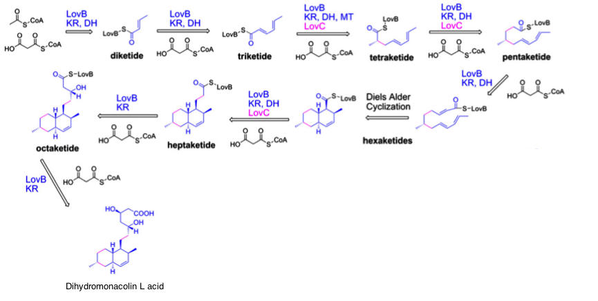
Figure) Synthesis of dihydromonacolin L by LovB and LovC

In the next step dihydromonacolin L acid is converted to monacolin J acid via the intermediate monacolin L acid by the enzyme lovA (source).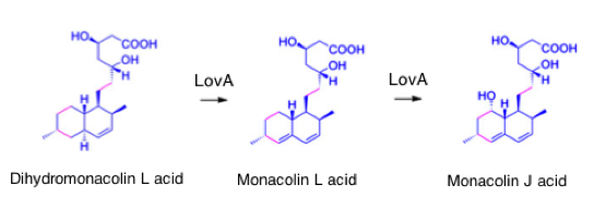

Figure) Synthesis of monacolin J by LovA

In parallel with this process there is another, very similar polyketide synthase, LovF, that synthesizes the intermediate 2-metylbutyryl-CoA from the same starting substrates, acetyl-CoA and malonyl-CoA.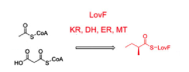

Figure) Synthesis of 2-methylbutyryl-CoA by LovF

In the final step of the process, LovD amalgamates monacolin J and 2-metylbutyryl-CoA into the product lovastatin.

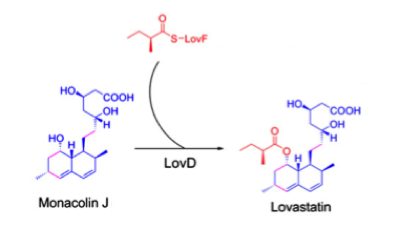
Figure) Synthesis of lovastatin by LovD

However, in order to balance the pathway more detail is required. It turns out that the co-factor NADPH is required by LovB, a non-trivial detail, which was found via Uniprot.

Results

In order to analyze the differences and compare the different models it is best to use a standardized namespace. Although MetanetX attempts to do so, it is not perfect and therefore one must carefully address the changed imposed by the system when one tries to upload a model. Another thing that needs to be taken into account is that the MATLAB script written is generic, such that when the models are modified the script should function properly as before.
Since the files are in SBML format (.xml), converting them to MATLAB (.mat) files allows for much faster loading and saving of the models. In order not to overwrite the previous model when saving it a prefix will be added to the file name click here for code . %chose the right path
modelPath = {'/Users/.../model1.xml','/Users/.../model2.xml,'/Users/.../model3.xml'}
modelPath = {'/Users/.../model1.mat','/Users/.../model2.mat,'/Users/.../model3.mat'}
modelPath = {'/Users/.../model1.sbml2.xml','/Users/.../model2.sbml2.xml,'/Users/.../model3.sbml2.xml'}

model = readCbModel(modelPath); % .xml files
load(modelPath{i}); % .mat files

modelNames = regexprep(modelPath{i},{'\.mat','.*/([^/]*)$'},{'.xml','new_$1'});
writeCbModel(model,'sbml',modelNames); % .xml files
save(modelNames,'model'); % .mat files

Converting and improving the A. terreus model

The A. terreus model was obtained in excel format. The first step taken is to convert the Excel file (.xls) into .xml format such that the model can be accessed via MATLAB: (link to script). For A. terreus the biomass reaction contained a great number of metabolites. By adding an additional compound to the reactions called 'BIOMASS' with a stoichiometric coefficient of 1, we can add an exchange reaction for biomass. This allows for optimization of this exchange reaction in FBA, a feature that should be generic for all models. The A terreus model does already contain a pathway for lovastatin production, however as it turns out this pathway is not functional. As it turns out the pathway is not balanced; the first step in which they lump the 35 reactions performed by lovB and lovC is missing the co-factor NADPH on one side, while NADP⁺ is present on the other.

J. Lui et al. (2013). Genome-scale reconstruction and in silico analysis of Aspergillus terreus metabolism. Molecular BioSystems, Vol. 9, p. 1939-1948

Standardising the models

Before proper conversion to the MNXM namespace from MetanetX can be finalized, uploading to model to MetanetX yields a mapping summary. This mapping summary includes information on the metabolites, compartments and reactions and their success of mapping. Since the system does not recognize all of them properly, the report has to be checked manually.

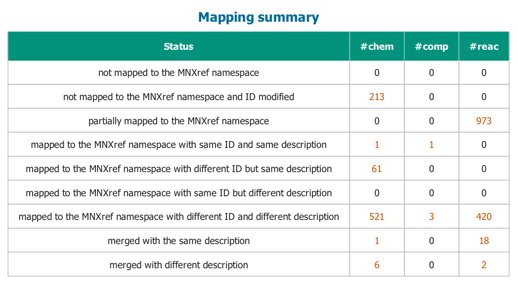
Figure) Mapping summary obtained after upload.

Metabolites
Mapping of metabolites is done on recognition of IDs and description. To check whether all metabolites were mapped correctly, mapping of those that do not have similar descriptions, IDs, or both, have to be manually curated from errors. Wrongly mapped metabolites had to be either set to their right respective MNXM id or else were given the prefix ‘my_’ to ensure proper mapping. click here for code . model.mets =
regexprep(model.mets,{'^COA\[','^ACCOA\[','^MALCOA\[','^NADPH\[','^NADP\[','^CO2\[','^H2O\[','^SAM\[','^SAH\[','^nadp\[','^accoa\[','^c160\[','^h2o\[','^coa\[','^hcya\[','^glcnt\[','^papce\[','^fgam\[','^sam\[','^co2\[','^sah\[','^malcoa\[','^nadph\['},{'MNXM12[','MNXM21[','MNXM40[','MNXM5[','MNXM6[','MNXM13[','MNXM2[','MNXM16[','MNXM19[','MNXM5[','MNXM21[','my_c160[','MNXM2[','MNXM12[','my_hcya[','my_glcnt[','pcace[','my_fgam[','MNXM16[','MNXM13[','MNXM19[','MNXM40[','MNXM6['});
model.mets =
regexprep(model.mets,{'^NADPLUS\[','^ACE\[','^PHACAL\['},{'NAD[','AC[','my_PHACAL['});
model.mets =
regexprep(model.mets,{'^COA\[','^OIVAL\[','^NADP\[','^CO2\[','^NADPH\[','^H2O\[','^ACCOA\['},{'MNXM12[','my_OIVAL[','MNXM5[','MNXM13[','MNXM6[','MNXM2[','MNXM21['});
model.mets =
regexprep(model.mets,{'^nadp\[','^accoa\[','^c160\[','^h2o\[','^coa\[','^hcya\[','^glcnt\[','^papce\[','^fgam\[','^sam\[','^co2\[','^sah\[','^malcoa\[','^nadph\['},{'MNXM5[','MNXM21[','my_c160[','MNXM2[','MNXM12[','my_hcya[','my_glcnt[','pcace[','my_fgam[','MNXM16[','MNXM13[','MNXM19[','MNXM40[','MNXM6['});

Compartments
To ensure mapping to the right compartment, it was found useful to put all the compartment names as a suffix behind square brackets (link to script). In a few cases mapping to the wrong compartment still occurred with several compounds that were not yet in the MNXM namespace, therefore these compounds were manually modified (link to script). Assignment of metabolite compartments , manual correction via excel and new names to prevent mis mapping of metabolites. %metabolite compartments
model.mets = regexprep(model.mets,{'m$','e$','p$','([^\]])$'},{'[m]','[e]','[x]','$1[c]'});
[newmets,newMNXM] = import_excel;
%function model= newname(model,newmets,newMNXM); %function

function [mets,MNXM] = import_excel

%% Import data from spreadsheet
% Script for importing data from the following spreadsheet % Workbook: /Users/.../correction.xlsx
% Worksheet: Sheet1
% To extend the code for use with different selected data or a different
% spreadsheet, generate a function instead of a script.

% Auto-generated by MATLAB on 2013/09/05 16:25:41

%% Import the data
[~, ~, raw] = xlsread('/Users/.../model.xlsx','Sheet1');
raw = raw(:,1:3);
raw(cellfun(@(x) ~isempty(x) && isnumeric(x) && isnan(x),raw)) = {''};
cellVectors = raw(:,[1,2,3]);

%% Allocate imported array to column variable names
mets = cellVectors(:,1);
metNames = cellVectors(:,2);
MNXM = cellVectors(:,3);

%% Clear temporary variables
clearvars data raw cellVectors;

end function model = newname(model,mets,MNXM)
mets = regexprep(mets,{'^M_','_[cmep]$'},{'',''});

for i=1:numel(mets)
if strcmp(MNXM{i},'')
model.mets = regexprep(model.mets,['^(' mets{i} '\[.*)'],'my_$1');
elseif strncmp(MNXM(i),'MNXM',4)
name = MNXM{i};
model.mets = regexprep(model.mets,['^' mets{i} '\['],[name '[']);
else
disp('unexpected entity')
end
end
Reactions
Similar to the A. terreus model, both A. niger and A. nidulans don’t have a exchange reaction for biomass, which was added to allow for optimization of this parameter with the same script for all models. The last non-triviality that had to be taken into account was the balancing of the reactions. To do so the model adds protons to the side of the reaction where it deems they are missing. A serious downside of this feature is that when metabolites are not recognized are involved, it is not able to take into account the protons absorbed or lost by these compounds. Still however, it adds protons to balance the reaction, but these are not rightly added. click here for code . compartments assigned to an unknown compartment. if i==4 %add biomass for terreus
model = addMetabolites(model,{'BIOMASS[c]'},{''});
model = removeRxns(model,{'BIOMASS'});
rxnFormula = '71.4 h2o[c] + 0.14613 asp[c] + 0.15371 glu[c] + 0.22294 ala[c] + 0.17484 gly[c] + 0.10126 gln[c] + 71.4 atp[c] + 0.08887 asn[c] + 0.15713 pro[c] + 0.03297 cys[c] + 0.16063 arg[c] + 0.05566 met[c] + 0.2067 ser[c] + 0.03822 trp[c] + 0.15021 thr[c] + 0.06317 his[c] + 0.09533 phe[c] + 0.07351 tyr[c] + 0.26575 chit[c] + 0.02795 utp[c] + 0.3348 mnt[c] + 0.03051 gtp[c] + 0.0015 glycogen[c] + 0.90068 13glucan[c] + 0.076 gl[c] + 0.07966 pc[c] + 0.06168 tagly[c] + 0.03399 pe[c] + 0.02264 my_paa[c] + 0.01378 ps[c] + 0.02091 ctp[c] + 0.16131 val[c] + 0.23243 leu[c] + 0.03153 my_ffa[c] + 0.00431 dgtp[c] + 0.00398 datp[c] + 0.00431 dctp[c] + 0.00398 dttp[c] + 0.12286 ile[c] + 0.1126 lys[c] -> 71.4 h[c] + 71.4 pi[c] + 71.4 adp[c] + 1 BIOMASS[c]';
model = addReaction(model,{'BIOMASS[c]','BIOMASSDEDUCED'},rxnFormula,[ ],[ ],[ ],[ ],1,'BIOMASS','',[ ],[ ],false);
end
biomass = model.mets(strcmpi(model.mets,'biomass[c]'));
if any(i==[2 3 4])
model = addExchangeRxn(model,biomass,-1000,1000);
end if i==1 %oryzae
model = removeRxns(model,{'r1068','r1069','r499','r500',},false,false);
rxnFormula = 'ATP[c] + GTP[c] -> AMP[c] + pppGp[x] +6 H[c]';
model = addReaction(model,{'r1068','GTP diphosphokinase'},rxnFormula,[ ],[ ],[ ],[ ],1,'GTP diphosphokinase','',[ ],[ ],false);
rxnFormula = 'H2O[c] + pppGp[x] + 4 H[c] <=> PI[c] + ppGp[x]';
model = addReaction(model,{'r1069','Exopolyphosphatase'},rxnFormula,[ ],[ ],[ ],[ ],1,'Exopolyphosphatase','',[ ],[ ],false);
rxnFormula = 'NADP[c] + 2 FERI[m] -> NADPH[c] + 2 FERO[m] + 4 H[m]';
model = addReaction(model,{'r499','NADPH-cytochrome p-450 reductase'},rxnFormula,[ ],[ ],[ ],[ ],1,'NADPH-cytochrome p-450 reductase','',[ ],[ ],false);
model = addReaction(model,{'r500','NADPH-cytochrome p-450 reductase'},rxnFormula,[ ],[ ],[ ],[ ],1,'NADPH-cytochrome p-450 reductase','',[ ],[ ],false);
end

if i==3 %niger
model = removeRxns(model,{'312'})
rxnFormula = '2 FERI[m] + NADP[m] -> 2 FERO[m] + NADPH[m] + 4 H[m]';
model = addReaction(model,{'312','NADPH-ferrihemoprotein reductase (cprA)'},rxnFormula,[],[],[],[],1,'NADPH-ferrihemoprotein reductase (cprA)','',[],[],false);
end

if i==4 %terreus
model = removeRxns(model,{'r0023'});
rxnFormula = 'fad[m] + hpro[c] -> fadh2[m] + phc[c] + h[c]';
model = addReaction(model,{'r0023','hydroxyproline oxidase'},rxnFormula,[],[],[],[],1,'hydroxyproline oxidase','',[],[],false);
end

Adding the lovastatin pathway

Since the lovastatin pathway is only present in the A. terreus model, but is not well balanced here, a function was written to add the pathway for lovastatin biosynthesis. First all the metabolites that are not yet in the model need to be added. Then the pathway upto the production of the intermediate dihydromonacolin L acid was added. This pathway consists of 35 reactions that have been lumped into 10 reactions. Together with the remaining 4 reactions required the total lovastatin biosynthesis pathway has been modeled in 14 steps. Finally also a exchange reaction for lovastatin was added to be able to optimise for its production.
The prefix 'Ex_' was added to all exchange reactions for easy recognition and an additional function was implemented that allows to easily change the optimisation criterion. Both the metabolites and reactions need to be added to the model. %add metabolites for lovastatin pathway
j =
{'diketide_LovBbound[c]','triketide_LovBbound[c]','tetraketide_LovBbound[c]','pentaketide_LovBbound[c]','hexaketide_LovBbound[c]','cyclic_hexaketide_LovBbound[c]','heptaketide_LovBbound[c]','octaketide_LovBbound[c]','nonaketide_LovBbound[c]','dihydromonacolin_L_acid[c]','monacolin_L_acid[c]','monacolin_J_acid[c]','2-metylbutyryl-COA[c]','lovastatin_acid[c]'};
h =
{'C4H5O','C6H7O','C9H13O','C11H17O','C13H19O','C13H19O','C15H23O','C17H27O2','C19H32O4','C19H32O4','C19H30O4','C19H30O5','C26H45N7O17P3S','C24H36O6'}; model = addMetabolites(model,j,h); %function
model = addLovPathway(model); %add reactions for lovastatin
model = addExchangeRxn(model,{'lovastatin_acid[c]'},0,1000); %add exchange reactions for lovastatin production
model.c(:) =0;
function model = addLovPathway(model)

metNames = {{'ACCOA','MALCOA', 'NADPH','diketide_LovBbound', 'NADP','COA','CO2','H2O'}, ...
{'MALCOA','diketide_LovBbound', 'NADPH','triketide_LovBbound','NADP','COA','CO2','H2O'}, ...
{'MALCOA','triketide_LovBbound','SAM','NADPH','tetraketide_LovBbound','SAH','NADP','COA','CO2','H2O'}, ...
{'MALCOA','tetraketide_LovBbound','NADPH','pentaketide_LovBbound','NADP','COA','CO2','H2O'}, ...
{'MALCOA','pentaketide_LovBbound','NADPH','hexaketide_LovBbound','NADP','COA','CO2','H2O'}, ...
{'hexaketide_LovBbound','cyclic_hexaketide_LovBbound'}, ...
{'MALCOA','cyclic_hexaketide_LovBbound','NADPH','heptaketide_LovBbound','NADP','COA','CO2','H2O'}, ...
{'MALCOA','heptaketide_LovBbound','NADPH','octaketide_LovBbound','NADP','COA','CO2'}, ...
{'MALCOA','octaketide_LovBbound','NADPH','H2O','nonaketide_LovBbound','NADP','COA','CO2'}, ...
{'nonaketide_LovBbound','dihydromonacolin_L_acid'}, ...
{'dihydromonacolin_L_acid','monacolin_L_acid'}, ...
{'monacolin_L_acid','H2O','monacolin_J_acid'}, ...
{'ACCOA','MALCOA','SAM','2-metylbutyryl-COA','COA','SAH','CO2','H2O'}, ...
{'2-metylbutyryl-COA','monacolin_J_acid','lovastatin_acid','COA'} ...
};
stoich = {[-1 -1 -1 1 1 2 1 1], ...
[-1 -1 -1 1 1 1 1 1], ...
[-1 -1 -1 -2 1 1 2 1 1 1], ...
[-1 -1 -2 1 2 1 1 1], ...
[-1 -1 -1 1 1 1 1 1], ...
[-1 1], ...
[-1 -1 -2 1 2 1 1 1], ...
[-1 -1 -1 1 1 1 1], ...
[-1 -1 -1 1 1 1 1 1], ...
[-1 1], ...
[-1 1], ...
[-1 -1 1], ...
[-1 -1 -1 1 1 1 1 1], ...
[-1 -1 1 1]};

for i=1:numel(stoich)
metNames{i} = strcat(metNames{i},'[c]');
metNames{i} = regexprep(metNames{i},' ','_');
model = addReaction(model,['rxnName' num2str(i)],metNames{i},stoich{i});
end

Medium constraints

In order to find medium constraints of the models all lower and upper bounds are first set to the value of -1000 and 1000 arbitrary units, respectively. Then one by one the lower and upper limit of the reaction bounds are set to 0 for one reaction at a time. If the model is not able to optimise the reaction of interest this indicates that exchange of this component with the medium is a prerequisite. If a lower bound larger then 0 is required this indicates that the component needs to be present in the in silico medium. When an upper bound larger then one required this means the opposite, namely that detrimental accumulation of this metabolite occurs ( See script ). function model = mediumCheck(model)

model.lb(findExcRxns(model))=-1000;
model.ub(findExcRxns(model))=1000;
er = find(findExcRxns(model));

for i=1:numel(er)
model.lb(er(i)) = 0;
check = optimizeCbModel(model);
if check.f<10^-6
display 'essential metabolite required, knowing:'
[model.rxns(er(i)) model.rxnNames(er(i))]
end
model.lb(er(i)) = -1000;
end
for i=1:numel(er)
model.ub(er(i))=0;
check = optimizeCbModel(model);
if check.f<10^m-6
display 'detrimental accumulation of'
[model.rxns(er(i)) model.rxnNames(er(i))]
end
model.ub(er(i)) = 1000;
end

Media

In order to define a proper in silico medium need to know which exchange reactions the models have in common and which of these are of essential importance.

Flux Balance Analysis

Gene knockout strategies

click here for code

blabla bla...

Team:Wageningen UR/Flux balance analysis