Team:Exeter/Modelling
From 2013.igem.org
(→Biological pathway simulation) |
(→Introduction) |
||
| Line 10: | Line 10: | ||
== Introduction == | == Introduction == | ||
| - | Our model predicts how the absorption spectrum of a modified ''E. coli'' changes over time in response to a given incident light spectrum. It | + | Our model predicts how the absorption spectrum of a modified ''E. coli'' changes over time in response to a given incident light spectrum. It can estimate key properties of the system such as stability, development time of the image, and the balance of colours. |
| - | The model is split into three sections. | + | The model is split into three sections. Initially, the reaction of each sensor species to a given incident light spectrum is calculated. This information feeds to the heart of the model, which involves simulating the biochemistry of our designed pathways. Finally the data from the simulation is used to plot the absorption spectrum of the system as it varies with time. |
Currently the model is based on results from literature and theoretical conjecture as experimental results are not available. The motivation for the model was to numerically characterize our bio-bricks for future use and to help us create the first colour coliroid. With experimental results the model could readily be updated to fulfill its original mandate. | Currently the model is based on results from literature and theoretical conjecture as experimental results are not available. The motivation for the model was to numerically characterize our bio-bricks for future use and to help us create the first colour coliroid. With experimental results the model could readily be updated to fulfill its original mandate. | ||
Revision as of 20:33, 4 October 2013
Modelling
Introduction
Our model predicts how the absorption spectrum of a modified E. coli changes over time in response to a given incident light spectrum. It can estimate key properties of the system such as stability, development time of the image, and the balance of colours.
The model is split into three sections. Initially, the reaction of each sensor species to a given incident light spectrum is calculated. This information feeds to the heart of the model, which involves simulating the biochemistry of our designed pathways. Finally the data from the simulation is used to plot the absorption spectrum of the system as it varies with time.
Currently the model is based on results from literature and theoretical conjecture as experimental results are not available. The motivation for the model was to numerically characterize our bio-bricks for future use and to help us create the first colour coliroid. With experimental results the model could readily be updated to fulfill its original mandate.
Control of bacteria using light has many applications. Di-chromatic control of bacteria has been achieved (REFERENCE) the challenge now is for Tri-chromatic control. Our lab project aims to produce a full colour ‘coliroid’ to demonstrate tri-chromatic control of bacteria. The modified E.coli are designed to carry three independent light sensitive pathways that each control the production of a specific pigment protein. The goal of which is to produce the world’s first colour bacterial photograph or ‘coliroid’. At time of writing there was nothing produced in the laboratory project with which to test our model.
A reliable computer model is essential for accurate implementation of tri-chromatic control. In the case of the theoretical bio-camera it is required to achieve an even balance of colours and optimum development time.
The model is based around KaSim, a stochastic simulator that reads Kappa, a rule based language. Stochastic simulation has the advantage over deterministic simulation because it replicates the random nature of brownian motion in cells more accurately. Rule based languages are particularly useful for biochemical signalling as the physical reactions are readily converted into digital rules. Matlab is used to process the signal from the incident light to the KaSim biochemcial signalling simulation. The outputs of which are processed by matlab to calculate the reflected light.
The Team
| | | |
Modelling Software
The model uses two programs; [http://www.mathworks.co.uk/products/matlab/ MATLAB®] and KaSiM. Together they provide the necessary tools to create an accurate model of our system.
KaSiM and Kappa
KaSiM is a [http://en.wikipedia.org/wiki/Stochastic stochastic] simulator that executes files written in [http://www.kappalanguage.org/ Kappa]. Kappa is a rule based modelling language for protein interaction networks. To download KaSiM or the manual please visit the KaSiM page.
KaSiM
Kappa
Rule-based languages describe a system by a governing set of rules. There is no change in the configuration of the system without the execution of a rule. Kappa is a high level langauge designed to describe protein interaction networks. There are 5 fundemental parts to the kappa language; agents, tokens, rules, rates and observables. It is essential to understand the roles each have in order to appreciate the stochastic model.
Agents and tokens
Agents and tokens represent the constituent molecules of a system. Agents are quantified in terms of their population number and are characterised having binding sites. Whereas tokens are quantified in terms of their concentration and do not have binding sites.
MATLAB®
[http://www.mathworks.co.uk/products/matlab/ MATLAB®] is a high-level language and interactive environment for numerical computation, visualization, and programming. It can be used to analyze data, develop algorithms, and create models and applications.
The model
The model describes the absorption spectrum of the cell as a function of time and a given time invariant incident light spectrum. This is achieved by calculating the effect of the known light input on the individual light sensitive proteins. This information is then fed into a stochastic simulation of the biological pathways that computes how the population of sensors and pigments vary over time. The total absorption spectrum over time is given by the sum of the product of every protein's population and the corresponding absorption spectrum of the protein. In this section each of these steps in considered in the following subsections.
It will be helpful to read the theory page and the modelling software section of this page before reading further as an understanding of the biological pathways and software is important for understanding the
Sensor activation rate calculation
The rule for each sensor is that it is either on or off. In the on state it catalyses the phosphorylation of the primary intermediate and in the off state it does not. Activation by light either turns a sensor on or off depending on the sensor species; the red and blue light sensors are switched off when activated while the green light sensor is switched on when activated. The activation rate is the forward rate of the rule that governs the state of a sensor. Its counterpart, the deactivation rate is the backward rate of the same rule.
The activation rate is calculated as the integral over all space of the product of the sensor's frequency response with the frequency spectrum of the incident light.
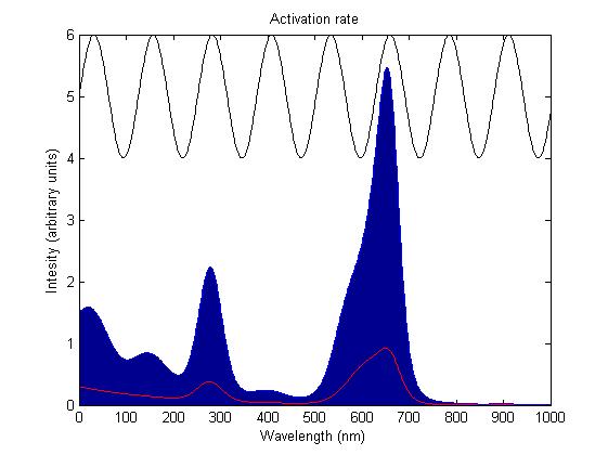
This has two important implications. Firstly it means that the sensor will not be activated by light that has no overlap between its spectrum and the frequency response of the sensor. Secondly there will be a saturation point at high intensity light where increasing the intensity will not appreciably affect the system as the activation rate will dominate the deactivation rate. Causing the sensors to be effectively permanently activated. These characteristics are faithful to the light sensitive proteins we are using and that is why we are using this method.
Biological pathway simulation
Our stochastic model is comprised of red, green and a blue light activated pathways. The pathways are independent in their signalling but share the common resources of the cell. Their biochemistry is represented by a series of rule. The rates of which were created to fit observations recorded in literature CITATION NEEDED. With experimental results this model can be readily updated to accurately describe our system.
INSERT DIAGRAM
The following section will include kappa jargon.
The kappa model describes in detail the pathway specific biochemistry and includes simplified descriptions of pathway related biochemistry. For example the controlled transcription and translation of pigment proteins is described in full but the constitutive transcription and translation of light sensor proteins is simplified.
The initial configuration has only DNA, RNA polymerase and ribosomes to transcribe and translate it. Every species of molecule except DNA is constitutively expressed. Every species of molecule except DNA, RNA polymerase and ribosomes has a spontaneous death rate. Every phosphorylated species has a spontaneous dephosphorylation rate.
Absorption spectrum calculation
Each protein species has an associated absorption spectrum. This multiplied by the population of the protein at a point in time gives the contribution of that protein to the total absorption spectrum of the cell at that moment. The sum of the contributions from each protein plus the absorption spectrum of the background cell gives the total absorption spectrum of the cell at that moment. This calculation repeated for every time step gives the total absorption of the cell over time.
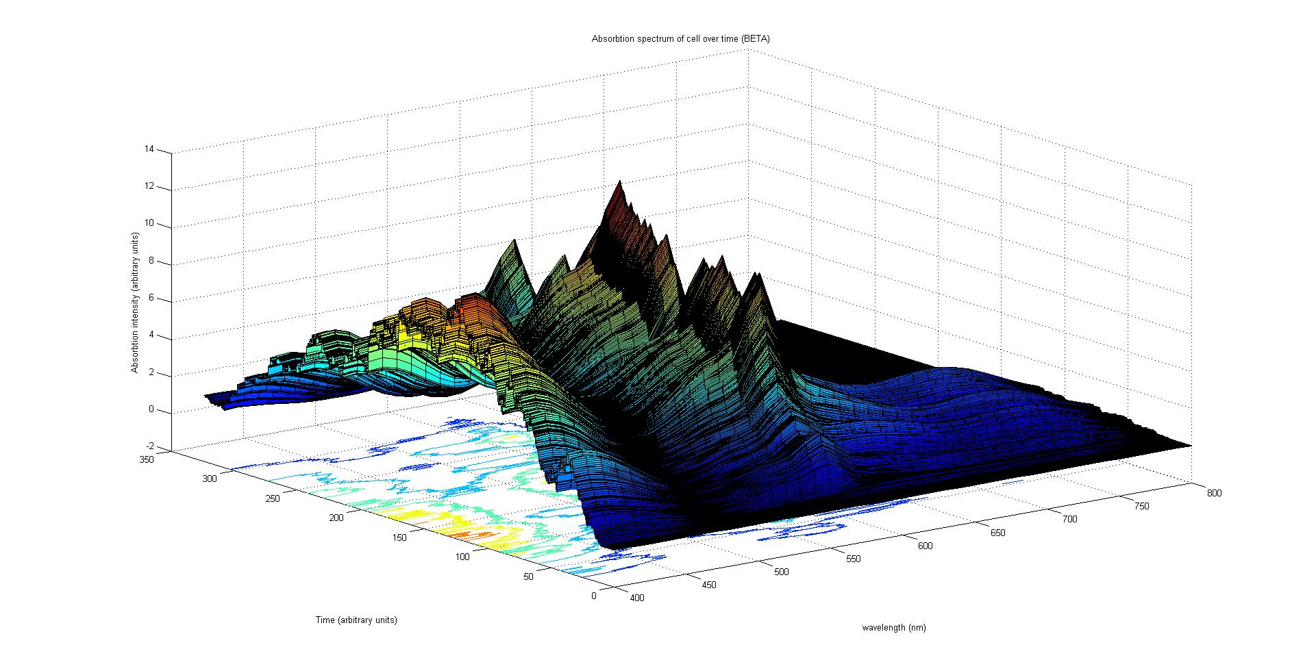
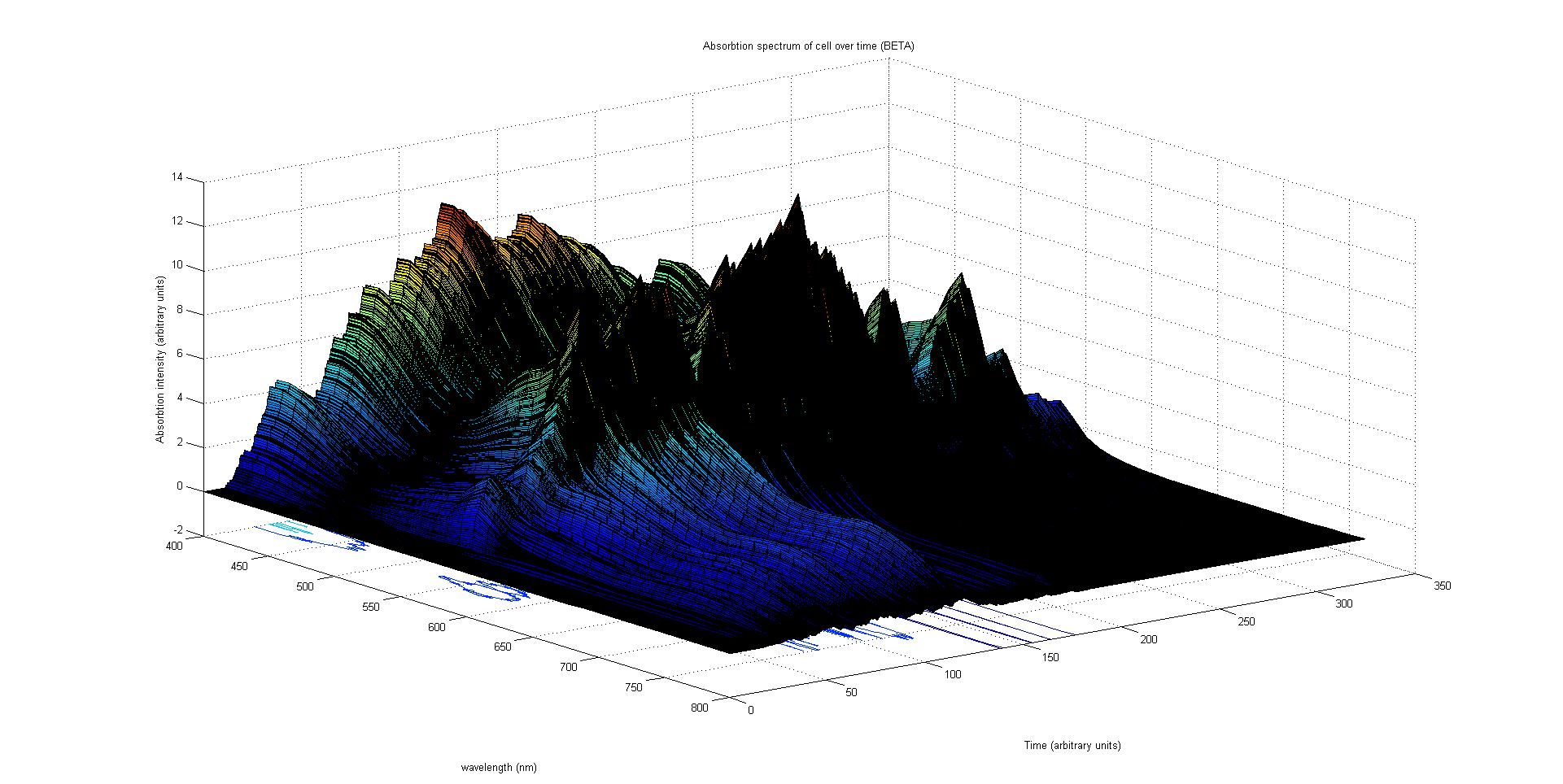
The absorption spectrum over time is plotted as a surface of intensity as a function of time and frequency.
The absorption spectrum at a point in time tells us what colour and tone the cell will be at that moment. Over time it shows us how the mix of colours change as the image develops, how long it takes to reach an equilibrium, the moment of greatest contrast and many other important features.
It will also reveal how the expression of a gene is controlled by each light sensitive pathway. Something which has implications for future projects.
Results
This section will list in detail the results of our model
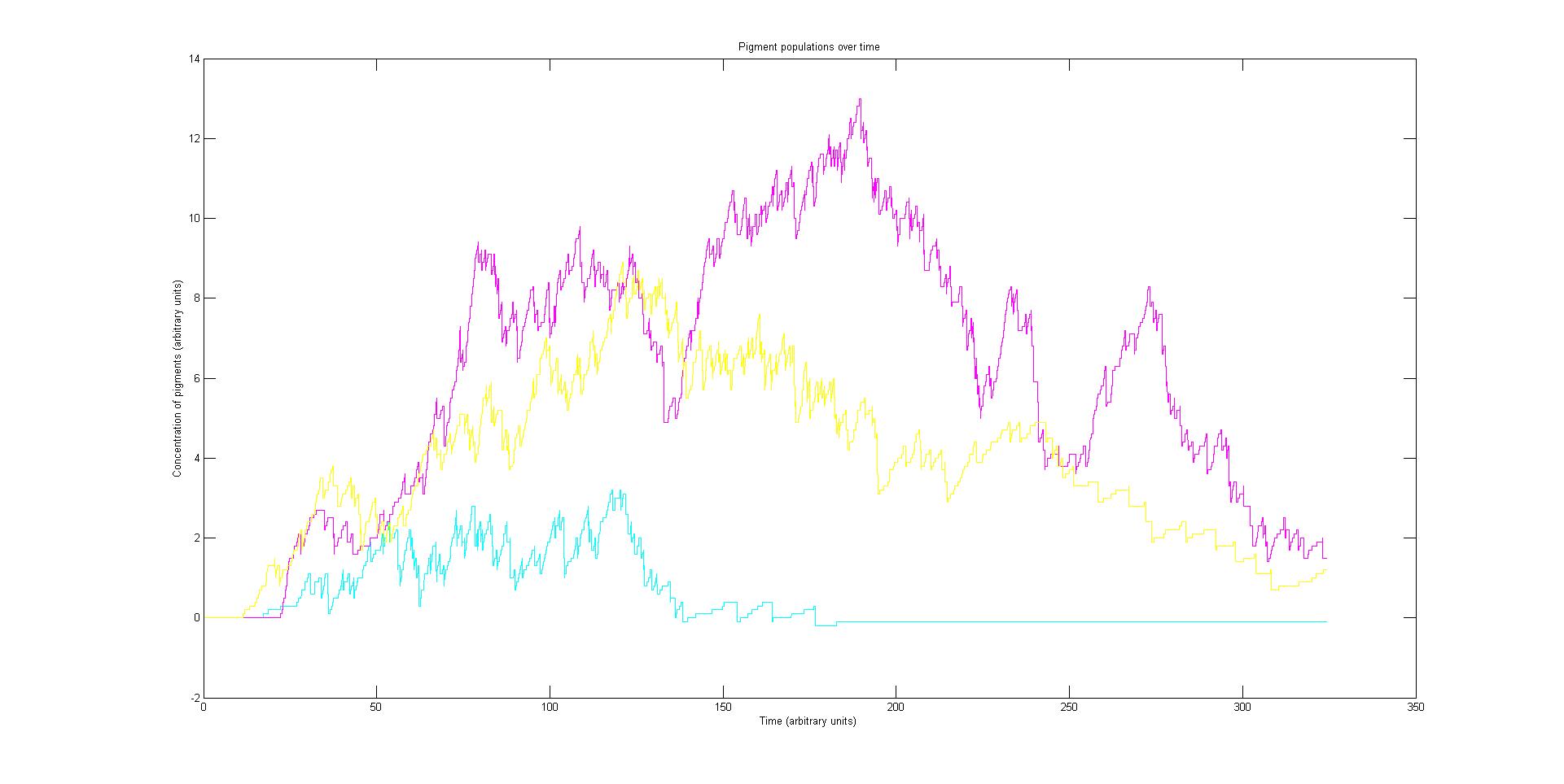
Preliminary results suggest that the mix of colours in an individual e.coli is very unpredicatable. But the average for a cohort of cells is more predicatable.
Analysis
This section will contain what the data means
Conclusions
This section will contain our conclusions about the model
Future
This section will contain our opinions about the future of the model
 "
"


