Team:Groningen/Modelling/21 August 2013
From 2013.igem.org
(Difference between revisions)
| Line 1: | Line 1: | ||
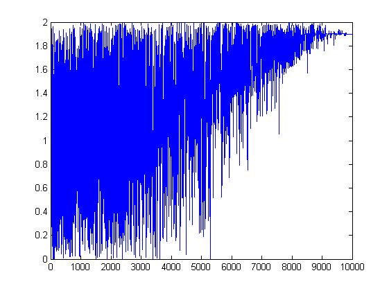
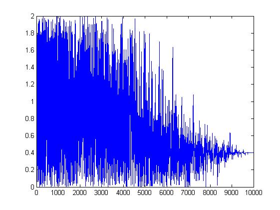
| - | Today we identified another faulty differential equation, and we implemented the simulating annealing algorithm for a dummy problem. The error function was simply the distance between some current value x and some goal y. The algorithm stabilizes around the goal as the time (or temperature) decreases, along with the degree of randomness. The plots below illustrate this for y = 1.9 and 0.4 respectively. The search space was any value between 0.0000 and 2.0000. | + | Today we identified another faulty differential equation, and we implemented the simulating annealing algorithm for a dummy problem. The error function was simply the distance between some current value x and some goal y. The algorithm stabilizes around the goal as the time (or temperature) decreases, along with the degree of randomness. The plots below illustrate this for y = 1.9 and 0.4 respectively. The search space was any value between 0.0000 and 2.0000. The main difference between this test problem and the real problem is that the search space will be bigger by a factor ~10^77, and that there will be more local optima. |
[[File:Goal1.jpg]] | [[File:Goal1.jpg]] | ||
[[File:Goal2.jpg]] | [[File:Goal2.jpg]] | ||
Latest revision as of 14:55, 21 August 2013
Today we identified another faulty differential equation, and we implemented the simulating annealing algorithm for a dummy problem. The error function was simply the distance between some current value x and some goal y. The algorithm stabilizes around the goal as the time (or temperature) decreases, along with the degree of randomness. The plots below illustrate this for y = 1.9 and 0.4 respectively. The search space was any value between 0.0000 and 2.0000. The main difference between this test problem and the real problem is that the search space will be bigger by a factor ~10^77, and that there will be more local optima.
 "
"

