"

From 2013.igem.org

Contents 1 Introduction 1.1 Switch modeling 1.2 Mass action modeling 1.3 Analytical modeling 1.3.1 Benefits 1.3.2 ERSESCO Algorithm 1.3.2.1 1. Equation 1.3.2.2 2. Reduction 1.3.2.3 3. Solution 1.3.2.4 4. Equilibration 1.3.2.5 5. Stabilization 1.3.2.6 6. Calibration 1.3.2.7 7. Optimization 1.4 SimBiology 1.5 Model of Recombinase Expression 1.6 Model of the Switch 1.7 Model of Inducible Hbif 2 Expression Model 3 Switch Model 4 Inducible Hbif Model 5 Future Directions

Introduction

Switch modeling

• produce both states of switch

• use model to optimize switch

Mass action modeling

Definition

• differential equations

• each equation is a sum of rates

• each rate is proportional to each of its reactants

Benefits

• can minimize assumptions

• already used in chemical rate equations

• standardizes equations:

    	• x is the species vector

    	• a is an amount of rates changing x

    	• b is a rate constant

    	• c is a number of different species involved

    	• d is a species involved

    	• e is a number of each species involved	

    	• f is a number of species d involved

    	• g is a highest species involved

    	• l is a rate order

    	• m is the highest number of rates involved

    	• n is the number of species

Analytical modeling

Benefits

• given parameters, it precisely predicts behavior

• accurately predicts the data needed to determine parameters (unlike numerical analysis)

• allows avoidance of numerical errors like rounding

• naturally standardized

ERSESCO Algorithm

The ERSESCO algorithm the Michigan team developed provides a clearly defined method of doing analysis on systems. The algorithm has seven major steps:

1. Equation

Formulate the system into a system of differential equations.

2. Reduction

Apply constraints, boundary conditions, and conservation laws to reduce the system of equations to fewer variables.

3. Solution

Solve the reduced system of equations, if possible.

4. Equilibration

Find the steady states of the system by setting differential equations to zero and solving for critical points.

5. Stabilization

Evaluate the Jacobian matrix of the system of equations at each critical point and find the corresponding eigenvalues. Eigenvalues with a negative real part are stable critical points.

6. Calibration

Solve for the parameters of the system of equations in terms of the system's initial, steady state, time-dependent variables. This step allows the system parameters to be easily characterized using experimental data.

7. Optimization

Optimize the steady state, eigenvalues, parameters, or other desired quantity by equating the derivative of that quantity with respect to each of the system's parameters with zero. Solving these equations gives the optimization conditions for that quantity.

SimBiology

SimBiology is a useful MATLAB package provided to all iGEM teams. It can be used as a tool to quickly run numerical approximations of biological systems whether or not data for system parameters are known. SimBiology can quickly produce a model from a simple schematic diagram. As a result, the package can quickly provide a qualitative analysis of a system with little work from the user.

In the following models, our team applied our ERSESCO algorithm to fully analyze the systems at hand, then a SimBiology simulation was used as qualitative verification.

Model of Recombinase Expression

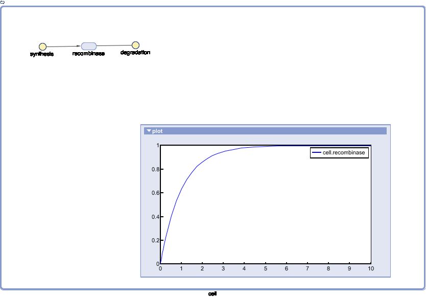
The Recombinase Expression Model describes the synthesis and degradation of any protein produced at a relatively constant rate. Here, the model is used in particular to describe the synthesis and degradation reaction rates ksyn and kdeg of recombinases in the cell. The model also predicts the recombinase concentration.

Model of the Switch

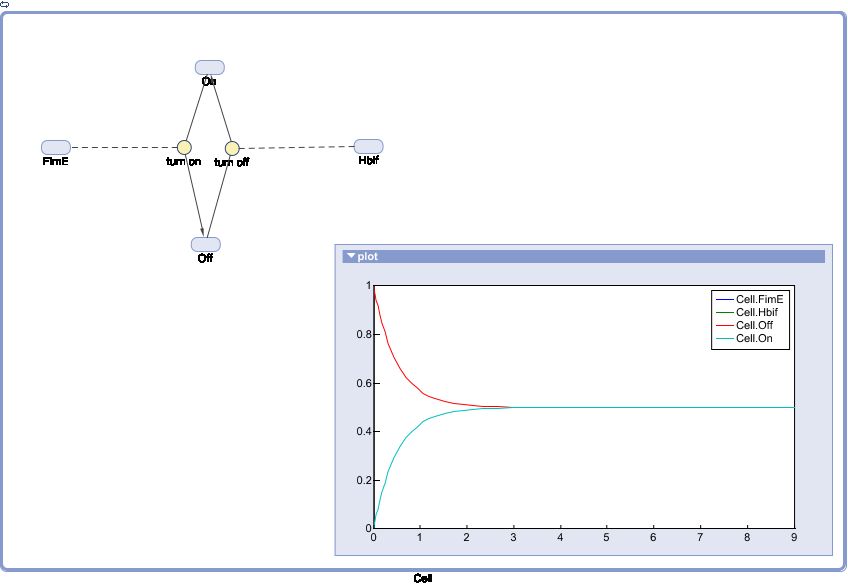
The Switch Model describes how the switch equilibrates when the concentrations of the recombinases FimE and Hbif approach constant values. This model assumes that each recombinase catalyzes a one way reaction. This model predicts the degree of cooperativity n and m in the binding reaction of the recombinase to DNA for FimE and Hbif, respectively. Furthermore, this model predicts the forward catalysis rate constants, kF and KH, for FimE and Hbif.

Model of Inducible Hbif

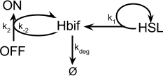
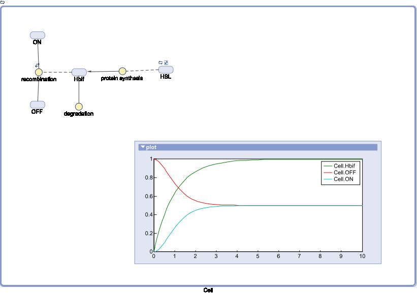
The Inducible Hbif Model describes how the switch flips when acted upon by the Lux/HSL-controlled expression of Hbif. In this model, [HSL] represents the concentration of the species HSL:pLux:LuxR, the complex that promotes the expression of Hbif. In this model [HSL] is a function of pLux and LuxR expression levels in the cell, the amount of HSL added, and the fractional occupancies at the complexation equilibrium. It can be assumed that this complexation reaction happens instantaneously with respect to the slow, rate-limiting translation step of Hbif. This model predicts the rate k1 of Lux-induced expression of Hbif, the degradation rate kdeg of Hbif, the forward and reverse rates k2 and k-2 of Hbif catalysis on the switch, and the equilibrium constant K2 for the switch when acted upon by Hbif.

Expression Model

Equation:

Reduction: None

Solution:

Equilibration:

Stabilization:

Calibration:

Optimization:

SimBiology:

Expression Model Derivation

Switch Model

Equation:

Reduction:

Solution:

Equilibration:

Stabilization:

Calibration:

Optimization:

SimBiology:

Switch Model Derivation

Inducible Hbif Model

Equation:

Reduction:

Solution:

Equilibration:

Stabilization:

Calibration:

Optimization of Hbif:

Optimization of ON:

SimBiology:

Inducible Hbif Model Derivation

Future Directions

Data!