Mathematical Modeling of Bistable Toggle Switch

Kinetic Model of Bistable System

Introduction to the Kinetic Model

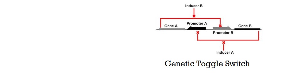
Tim Gardner from Jim Collins' Lab at Boston University published one of the first major papers on genetic toggle switch (Gardner 2000). In his work, he used a kinetic approach to model the stability of a genetic toggle switch. His equations involved two equations expressing the change in the level of two mutually repressive repressors with respect to time, and he showed how strength of promoters and cooperativity affects the stability of the toggle switch system using bifurcation diagrams and nullclines.

Based on his approach of using bifurcation diagrams and nullclines, we decided to develop our kinetic model and test it in a similar approach. Two main tools used in our model were nullclines and bifurcation diagrams. Nullcline, also called zero-growth isocline, is a line that represents the set of points at which the rate of change is zero. In the context of genetic toggle switch, nullclines show where rate of change of repressor 1 (U) and repressor 2 (V) are zero. It is clear that at the intersection of these two nullclines are steady-state points of the system because these are points where the change of both repressor levels with respect to time is zero.

Shown below are examples of nullclines we have generated using a system of two rate equations for U and V from Gardner's work (Gardner 2000). The difference between the two figures with nullclines on left and right is that the system on the left is bistable with the system on the right is mono-stable. Plot on the left shows that there are two stable steady-states where only one of the two repressors exists at a high level, inhibiting the production of the other repressor. There is a third intersection in the middle, however, this point can be mathematically shown to be unstable using the eigenvalue of the Jacobian matrix involving U and V (Strogatz, 2001). The value of U and V does not change exactly at this unstable steady-state, however, the level of repressors will quickly diverge from this point even at the smallest perturbation. The figure on the right shows that at a different combination of parameters, a system can be mono-stable where the nullclines only intersect once at a stable steady-state solution.

In addition to the nullclines, the plots show the trajectories of how points with different initial conditions on the level of U and V end up at either of the two stable steady states. All the trajectories are color-coded in terms of where they eventually end up--the line across the middle labeled as "separatrix" separates the initial conditions that lead to one solution from the initial conditions that lead to the other solution. Two interesting observations can be made. First, some trajectories reach close to the unstable-steady state but when it gets very close to it, it quickly diverges to either of the two stable steady-state solutions. Secondly, the plot on the right shows that when the set of promoters are chosen appropriately, the system becomes monostable and all initial points end up at the single stable steady-state solution. As such, nullclines can confirm the bistability of a toggle switch system.

Another type of graphs used in our kinetic modeling approach is bifurcation diagrams. Bifurcation is a mathematical term that describes a phenomenon "when a small smooth change made to the parameter values (the bifurcation parameters) of a system causes a sudden 'qualitative' or topological change in its behavior" (Blanchard et al 2006). In terms of a system with two mutually repressive genes, bifurcation occurs when the system changes its stability—switching between monostability and bistability. In a bifurcation diagram, the lines indicate the set of all points where bifurcation occurs, and the two regions delineated by bifurcation lines represent the monostable and bistable regions. Whereas Gardner showed the effect of change in cooperativity on the bistable region, our kinetic approach uses bifurcation diagrams show how promoter strength, repressor binding strength, and basal expression level affect the stability of the system.

Development of Our Kinetic Model

With the understanding of nullclines, bifurcations, and their meaning on a system of two mutually repressive genes, we have created our own kinetic model with the purpose of exploring the conditions necessary for a system to be bistable. Our model shown below incorporates the P_bound term from our thermodynamic model. In this sense, this model is a combination of kinetic and thermodynamic model. As mentioned before, a key assumption in this model is that the gene expression is directly proportional to the probability of RNAP bound to the promoter. Also, same values for used for variables that appeared in the thermodynamic model (i.e. P, N_ns, Kb, T,...). If we assume that our repressors are never actively degraded, the only way to decrease its concentration is by dilution due to cell growth. This assumption links the degradation rate (more precisely, dilution rate) (δ) to the growth rate of the yeast. Further, if we also assume exponential growth, ln(2)/90 is the growth rate of S.cerevisiae dividing every 90 minutes. As such, ln(2)/90 was used as the value of δ throughout the model.

Our kinetic model assumes five repressor binding sites and that there exist a basal level of gene expression even at maximum repression (phenomenon which we will call "leakiness" of the promoter). Whereas Gardner's model uses promoter strengths and cooperativity of repression as parameters to control the bistable regions, this model includes a lot more parameters: for example, promoter strength, leakiness of promoter, strength of repressor binding, and number of binding sites. Also, our model uses the probabilistic P_bound term which models what actually happens during gene expression: physical binding of RNAP to the promoter. In this sense, our model is more comprehensive and more mechanistic and the previously suggested model by Gardner.

A plot of nullclines and trajectories was produced using our kinetic model. The plot above shows two nullclines that intersect and three points, two of which are stable steady-state solutions and one of which is an unstable-steady state. This graph confirms that our model, which combined thermodynamic and kinetic approaches, could demonstrate a bistable system when given appropriate parameters. In the subsequent section, our kinetic model was the tested with various combinations of parameters to test how these changes affect the bistable regions, and thus the stability of the system.

Results from Our Kinetic Model

Our model was used to demonstrate the effect of changing various parameters on bistable regions of the system. Specifically, the strength of promoters, combination of strong and weak binding repressors, and basal rate of gene expression (leakiness of promoters) were changed. The parameters changed, their values, and their meanings are tabulated below. Bistable regions for the different parameters were plotted and are also shown below. Note that the axes of the plots are not promoter strengths but binding strengths of the two repressors. Using these values on the axes, we could see how the constraints on the strength of repressor binding to achieve bistability changed.

This plot shows that the bistable region shrinks when the strength of one promoter is decreased. When a promoter is weak, the repressor binding strength must be high to achieve a bistable system. This result can be explained by the fact that weaker promoter leads to lower level of repressors, and that stronger binding strength is required to achieve the same level of repression with a lower repressor level.

In this plot, a combination of weak and strong binding were used to demonstrate the effect of unbalanced binding strengths on the bistable region. As the number of weak binding increased, the bistable region shrunk diagonally. This result is intuitive in that increasing the number of weaker binding requires stronger repressors to achieve the same level of repression and thus maintain bistability.

Finally, the effect of increasing the leakiness of a promoter is shown here. Interestingly, as a promoter becomes leakier, the boundary of the bistable region curves inwards and forms an enclosed shape. This result is reasonable because when a repressor is extremely strong, even low basal level of expression can have strong repression of the other gene, thus leading to monostability.

Therefore, we have demonstrated the effect of various parameters on the bistable regions for a set of two mutually repressive genes. Our results show how the bistable region decreases with decreasing promoter strength, weaker binding, and leakier promoter; these results consequently suggest the range of possible values for the dissociation constants of the two repressors that can lead to bistability. From the results of both thermodynamic model and the kinetic model, we now have a theoretical guide to constructing a genetic toggle switch; a guide that can be used to couple two genes that have the optimal combination of cooperativity, number of binding sites, binding strengths, promoter strengths and leakiness.

Mathematica Code

The Mathematica codes used for the thermodynamic model can be found here.

References

1. Gardner T, Cantor C, Collins J: Construction of a genetic toggle switch in Escherichia coli. Nature 2000. 403:339-342.
2. Strogatz S: Nonlinear dynamics and chaos. 2001. Westview Press.
3. Blanchard P, Devaney R.L, Hall G.R: Differential Equations. 2006. London: Thompson. pp. 96–111.

Navigate

Modeling Pages

1. Cooperativity and Hill Equation
2. Thermodynamic Model: Introduction
3. Thermodynamic Model: Application
4. Kinetic Model (You are here)

Supplementary Materials

1. Derivation of the Thermodynamic Model
2. MATLAB/Mathematica Codes Used