 "
"
Team:Groningen/Modeling/Heatmotility
From 2013.igem.org
| Line 127: | Line 127: | ||
<p>We know that in normal steady state conditions, the chance of flagella spinning CCW is 0.65, so that P(CCW) = 0.65 and P(CW)=0.35 [x7]. We also know that the average swim period is ~1.02 seconds and the average tumble period 0.165 seconds [x8], so that for every 100 ms the chance of swimming given a swimming state is 0.903%, and the chance of tumbling given a tumbling state is 0.6061, which is to say: P(S|S)= 0.903 and P(T|T)= 0.6061. We also know that when CCW=0, that P(S|S)=1 and P(T|T)=0, and that when CCW=1, that P(S|S)=0 and P(T|T)=1.</p> | <p>We know that in normal steady state conditions, the chance of flagella spinning CCW is 0.65, so that P(CCW) = 0.65 and P(CW)=0.35 [x7]. We also know that the average swim period is ~1.02 seconds and the average tumble period 0.165 seconds [x8], so that for every 100 ms the chance of swimming given a swimming state is 0.903%, and the chance of tumbling given a tumbling state is 0.6061, which is to say: P(S|S)= 0.903 and P(T|T)= 0.6061. We also know that when CCW=0, that P(S|S)=1 and P(T|T)=0, and that when CCW=1, that P(S|S)=0 and P(T|T)=1.</p> | ||
| - | <p>These points are used to fit two curves (Eq XX and XX), which can be used to describe the threshold for switching from a tumbling state to a swimming state, and vica versa. The curves are plotted below as a function of P( | + | <p>These points are used to fit two curves (Eq XX and XX), which can be used to describe the threshold for switching from a tumbling state to a swimming state, and vica versa. The curves are plotted below as a function of P(CWW). </p> |
<p>place equations here</p> | <p>place equations here</p> | ||
Revision as of 19:31, 3 October 2013
Heat Motility
The goal for our heat motility system is to obtain higher concentrations of silk in close proximity to the implant. This is achieved by immobilizing the silk producing bacteria once they are within some distance to the implant, which is enabled by integrating the standard chemotaxis system with the DesK membrane fluidity sensor system. The result is that B. subtilis stops moving when it is 37°C, and swims when it is 25°C. In our model we simulate the behavior of these systems and, if necessary, implement biologically plausible modifications to make it feasible.The chemotaxis system of B. subtilis
We first setup a model for the standard chemotaxis system. This system enables bacteria to seek out areas of higher concentrations of nutrients by modifying the direction of flagella rotations as a response to changes in concentrations of attractants and repellents. An increase in the concentration of attractants results in more clockwise (CCW) rotations, and an increase in the concentration of repellents in more counter clockwise (CW) rotations, which corresponds to an increased chance of swimming straight and tumbling respectively. This effect is complemented by the systems essential ability to adapt to any concentration of attractant or repellent. Given a homogenous environment, the system will therefore allways maintain the same swimming to tumbling ratios.
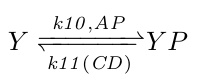
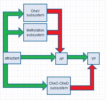
At the molecular level the flagella behavior is controlled directly by the concentration of phosphorylated CheY (YP): more YP results in more CCW rotations (more swimming) and less YP in more CW rotations (more tumbling). YP is controlled by phosphorylated CheA concentrations (AP), its natural decay rate, and by CheC_CheD complex concentrations (CD), which act as YP phosphorylases. Because the natural and CD induced YP decay rates are unknown, we combined them by making the k11 rate coefficient a function of CD with the natural YP decay rate as its offset.
|
| Figure 1 |
In order to obtain proper swimming behavior, we require an initial increase and a delayed decrease in YP. The initial YP increase is due to an in increase in AP (which donate their phosphor groups to CheY) as a response to increased attractant concentrations. The decrease in YP is realized by two negative feedback systems (the CheV and the methylation subsystem), which decrease CheA phosphorylation rates, and by one negative feedfoward system (the CheC-CheD subsystem), which increases the YP decay rate.
|
| Figure 2 |
CheA phosphorylation
Inside the cell CheW, CheA and CheV form complexes with the inter-membrane receptor protein. When attractants bind to the receptor, CheA undergoes a change in conformation that enables it to be phosphorylated.
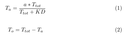
Following the example of David C. and John Ross [x1], we assume the binding and dissociation of attractants with their receptors is fast, and that it can be described with the equilibrium equation (1), where KD is the dissociation constant for the aspartate receptor (which is focus of this model). The concentration of unbound receptors is then given by (2).
|
| Figure 3 |
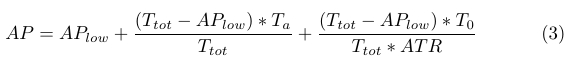
Due to high concentrations of ATP in the cell, we assume similar kinetics for the CheA phosphorylation rate. It then follows that the positive increase in AP levels is proportional to bound receptor (Ta) and unbound receptor (T0) levels, and can be described by (3), where ATR is a constant.
|
| Figure 4 |
The CheV subsystem
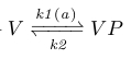
The first adaption system of B.subtilis, the CheV subsystem, contributes to a delayed decrease in YP through a decrease in AP. This is realized by phosphorylated CheV (VP), which obtains its phosphor group from AP, after which it may disrupt the bond between the attractant-bound receptor and CheA, hereby inhibiting CheA phosphorylation [x2].
Because AP levels are proportional to attractant levels we neglect the AP in our reactions (chem reaction 2) and take the rate coefficient k1 as a linear function of attractant levels (fig x). This disrupts the feedback loop between AP and VP, and makes the optimization later easier (see 'Parameters And Optimization' section).
|
| Figure 5 |
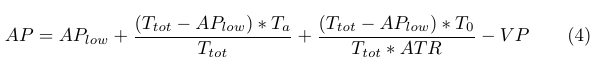
The negative decrease in AP due to VP is approximately 22% of the positive increase in AP described in (3), and is incorporated into the AP formula by subtraction (4).
|
| Figure 6 |
The methylation subsystem
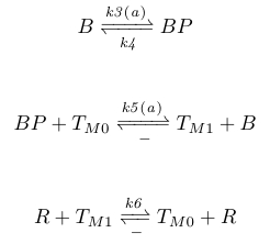
The second adaption system of B.subtilis is the methylation system, which regulates the CheA phosphorylation rate through phosphorylated CheB (BP) and CheR. After obtaining its phosphor group from AP, BP can shuffle methyl groups between different receptor residues. It is thus proposed that the methylation of certain receptor residues can activate the receptor, whilst the methylation of others can deactivate it [x2].
In order to provide negative AP feedback, BP would then shuffle methyl groups on the activation residues to the deactivation residues, whilst CheR shuffles methyl groups from the deactivation residues to the activation residues. We describe this system with the chemical reactions given below, where TM0 represents the methyl-deactivated receptors and TM1 the methyl-activated receptors.
|
| Figure 7 |
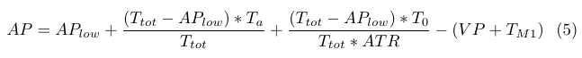
Rate coefficients k3 and k5 are again linear functions of attractant concentrations, which enables us to eliminate the feedback loop involving AP, BP, and TM1, and it justified by the fact that AP is proportional to attractant levels. The negative AP feedback involving TM1 is incorporated into equation (4) simply by subtracting TM1 from AP, and is given by (5). The total amount of negative AP feedback is approximately 35% of the positive increase.
|
| Figure 8 |
The CheC-CheD subsystem
The third adaption system of B.subtilis involves the CheC and CheD chemotaxis proteins. As of yet there appears to be no consensus on the exact behavior of this system. Christopher V. Rao. et al (2008) propose two viable options; a negative feedback and a negative feedfoward system.
In the negative feedback system YP binds to CheC and CheD to form a complex. In doing so, it may pull receptor-bound CheD from the receptor where it functions as a stimulatory protein with respect to CheA phosphorylation. In this system, YP is therefore decreased through AP by means of CheD removal.
In the negative feedfoward system, CheD is also bound to the receptor, but it no longer has its stimulatory function. Instead, it is released from the receptor upon the binding of attractant, after which it may form a complex with CheC where it functions as a YP phosphatase.
Contrary to Christopher et al (2008), we propose that the negative feedfoward system is the more likely case since the negative feedback system includes a time extensive feedback loop involving AP and YP through CheC, CheD, and the receptors. In our test simulations (not presented here), we observed adaption times of up to 10 minutes, whilst wild typ B.subtilis adaption times are approximately one minute [x6].
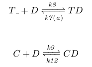
The chemical reactions for this negative feedfoward system can be seen below, where TD is the concentration of receptors with CheD bound, T_ the concentration of receptors with no CheD bound, and C CheC. We furthermore model the receptors change in conformation, and the following CheD release, by taking k7 as a non-linear function of attractant levels with an offset equal to its CheD release rate with no stimulatory ligand bound.
|
| Figure 9 |
Parameter optimization
Although the rate coefficients and molecular concentrations of the chemotaxis system in E.Coli are relatively well documented, for B.subtilis they are mostly unknown. Where possible, we therefore adopt values from the E.Coli chemotaxis system, for which Li and hazelbouwer (2008) have measured the following molecular concentrations: CheA+AP=5.3µM, CheB+BP=0.28µM, CheY+YP=9.7µM, and CheR=0.16µM.
We now assume that CheA and CheV are saturated with respect to the formation of receptor complexes with CheW and the intermembrane receptor protein. We further assume that the conserved molecular concentrations of CheD are equivalent to CheA, so that we can state the following: CheV+VP = CheA+AP = Ta+T0 = TD+T_ = TM1+TM0 = CD+TD+D = 5.3µM
To find appropriate values for the rate coefficients we applied the simulated annealing algorithm. This is a heuristic-driven & probabilistic optimization algorithm that can be used to find optimal solutions for complex problems. In our case, we require the algorithm to find the set of parameters that enable exact adaption of YP concentrations.
Before we can apply the algorithm, we must define an error function. The error function determines what will be optimized, as it is the result of this function that the algorithm will strive to minimize. Because we are interested in the steady state value of YP, we require all molecular values to be in equilibrium before any further assesment can be established. The core of the error function for some set of parameters is therefore defined as the distance of each molecular concentration from its equilibrium value.
We first applied the algorithm to the CheV subsystem for attractant levels 0 and 5.8 (saturation). The error function was defined as the distance of each molecular concentration from its equillibrium value, along with the requirement that the total amount of negative AP feedback was 20 to 40% of the total attractant-induced AP increase. The same procedure was applied to the methylation subsystem, and, finally, to the system as a whole, where the previously optimized parameters were ofcourse not further optimized. The error function was also modified to ensure that the YP equillibirum was constant across all levels of attractant ranging from 0 to 5.8.
Exact adaption
We used matlabs ode45 function to simulate the differential equations for different levels of attractant. The simulations show how YP reactes to the addition and removal of different levels of attractant, which correspond to B.subtilis swimming and tumbling along increasing and decreasing gradients of attractant respectively. The tumbling along the decreasing gradients ensures that the bacteria will not swim deeply into undesirable areas, but will instead tumble at the edge until adaption has taken place, and it resumes its standard run and tumble behavior. Because it is still on the edge of the more desireable region it will have a higher chance of falling back in, after which YP will again increase so that B.subtilis can swim deeper into the nutrient rich area.
Figure x1
Figure x2
Motility model
Before we can simulate the swimming behaviour of B.subtilis we need to relate YP to flagella rotations, for which we use the formula provided by Kuo and Koshland (1989) (6), where h is a constant we use to fit our steady state YP value to data.

|
| Figure 10 CHANGE TO CWW! |
We know that in normal steady state conditions, the chance of flagella spinning CCW is 0.65, so that P(CCW) = 0.65 and P(CW)=0.35 [x7]. We also know that the average swim period is ~1.02 seconds and the average tumble period 0.165 seconds [x8], so that for every 100 ms the chance of swimming given a swimming state is 0.903%, and the chance of tumbling given a tumbling state is 0.6061, which is to say: P(S|S)= 0.903 and P(T|T)= 0.6061. We also know that when CCW=0, that P(S|S)=1 and P(T|T)=0, and that when CCW=1, that P(S|S)=0 and P(T|T)=1.
These points are used to fit two curves (Eq XX and XX), which can be used to describe the threshold for switching from a tumbling state to a swimming state, and vica versa. The curves are plotted below as a function of P(CWW).
place equations here
place functions here
Homogenous and non-homogenous environments

|
| Figure 15 |

|
| Figure 16 |
CheC knockout
The effects of temperature
The DesK system
Demonstration
Parameters and differential equations
| Protein concentrations | Value | Reference |
|---|---|---|
| Y+YP | 9.7µM | [x5] |
| B+BP | 0.28µM | [x5] |
| CheR | 0.16 | [x5] |
| A+AP | 5.3µM | [x5] |
| Ta+T0 | 5.3µM | - |
| V+VP | 5.3µM | - |
| CheD+CD+TD | 5.3µM | - |
| TD+T_ | 5.3µM | - |
| TM0+TM1 | 5.3µM | - |
| CheC+CD | 3.9686µM | Optimized value |
| Rate coefficients | Value | Reference |
|---|---|---|
| k2 | 2.79937 | Optimized value |
| k4 | 3.21494 | Optimized value |
| k6 | 0.74553 | Optimized value |
| k8 | 0.09981 | Optimized value |
| k9 | 0.04779 | Optimized value |
| k10 | 0.11346 | Optimized value |
| k12 | 1.39741 | Optimized value |
| Dependent rate coefficients | Function |
|---|---|
| k1 | blabla k1 function |
| k3 | blabla k3 function |
| k5 | blabla k5 function |
| k7 | blabla k7 function |
| k11 | k11_basal + k11_scale*CD |
| Constants | Value |
|---|---|
| k11_basal | zzzzzzzzzzzzzz |
| k11_scale | zzzzzzzzzzzz |
| ATR | zzzzzzzzzzz |
| KD | 0.5 |
Matlab code
References
[x2] the three adaption systems of b subtilis [x5] Li and hazelbouwer (2008) [x6] http://www.rpgroup.caltech.edu/courses/PBoC%20ASTAR/files_2011/articles/BergSourjikPNAS.pdf [x7] model of excitation and adaption [x8] Berg and Brown (ref in x7)

|
| Figure 11 |

|
| Figure 12 |

|
| Figure 13 |

|
| Figure 14 |