 "
"
Team:SYSU-China/Project/Modeling
From 2013.igem.org
| (31 intermediate revisions not shown) | |||
| Line 58: | Line 58: | ||
<DIV class="chapter"> | <DIV class="chapter"> | ||
<span>Project/Modeling</span> | <span>Project/Modeling</span> | ||
| - | |||
| + | |||
| + | <h1> 1.Overview </h1> | ||
<p> | <p> | ||
Modeling is a powerful tool in synthetic biology and engineering. In the iPSCs Safeguard | Modeling is a powerful tool in synthetic biology and engineering. In the iPSCs Safeguard | ||
| - | |||
project, modeling has provided us with an important engineering approach to characterize our | project, modeling has provided us with an important engineering approach to characterize our | ||
| - | |||
pathways and predict their performance, thus helped us with modifying and testing our | pathways and predict their performance, thus helped us with modifying and testing our | ||
| - | |||
designing. | designing. | ||
</p> | </p> | ||
<p> | <p> | ||
| - | Basically, the models built by us can be divided into two levels. On | + | Basically, the models built by us can be divided into two levels.On gene level, we hope to gain insight of the gene expression dynamics of our |
| + | whole circuit. And also we tried to better characterize our parts, analyze our experimental data, for all of the sensor, switch, and the killer. | ||
| + | |||
| + | Several tools including ODEs and interpolation are employed. | ||
| + | </p> | ||
| + | <p> | ||
| + | On cell level, we proposed | ||
the multi-compartment model to trace the change of the iPS cells in different time nodes, | the multi-compartment model to trace the change of the iPS cells in different time nodes, | ||
| - | |||
thus we are able to describe the growth and decay of iPSCs. The number of cells at the | thus we are able to describe the growth and decay of iPSCs. The number of cells at the | ||
| - | |||
initial stage, growth rate and death rate of cells caused by suicide gene in our Safe-guard | initial stage, growth rate and death rate of cells caused by suicide gene in our Safe-guard | ||
| - | + | pathway were all taken into account. | |
| - | pathway were all taken into account | + | |
| - | + | ||
| - | + | ||
</p> | </p> | ||
| - | |||
| - | |||
| - | |||
| - | + | <h1>2.Gene expression dynamics of iPSC Safeguard</h1> | |
| - | + | <h2>2.1 analysis of the problem</h2> | |
| - | + | ||
| - | + | ||
| - | + | ||
| - | + | ||
| - | + | ||
| - | + | ||
| - | <h1> | + | |
| - | </h1> | + | |
| - | <h2> | + | |
| - | </h2> | + | |
<p> | <p> | ||
| - | + | Firstly we built a model to help ourselves better understand the gene expression dynamics of the whole circuit. In our device, tTA protein is | |
| - | expressed by a | + | firstly expressed by a EF1-α promoter and will then bind to TRE element, activating transcription of gene of interest, in our case suicide gene or |
| - | + | GFP. This process is affected by the Dox suppression effect. And the TRE element alone without tTA protein has a leaky expression. After production | |
| - | + | and functioning, the protein of interest will undergo degradation. And to simplify the model, we consider the miRNA degradation effect as part of | |
| - | + | this process. | |
| - | + | ||
| - | + | ||
| - | + | ||
| - | + | ||
</p> | </p> | ||
<p> | <p> | ||
| - | + | Then we wrote down the four chemical reactions in represent of each process. | |
| - | + | ||
| - | the | + | |
| - | + | ||
| - | + | ||
| - | + | ||
| - | + | ||
</p> | </p> | ||
| + | <br/><img src="https://static.igem.org/mediawiki/2013/0/0a/New_model_1.png" width="200" /><br /> | ||
<p> | <p> | ||
| - | + | The symbol declaration is: | |
| - | + | ||
| - | + | ||
</p> | </p> | ||
| - | |||
| - | |||
| - | |||
<p> | <p> | ||
| - | X1: | + | X1:tTA protein |
</p> | </p> | ||
<p> | <p> | ||
| - | + | D: the TRE promoter | |
</p> | </p> | ||
<p> | <p> | ||
| - | + | X1D:the tTA-TRE complex | |
</p> | </p> | ||
<p> | <p> | ||
| - | + | X2: the protein of interest | |
</p> | </p> | ||
<p> | <p> | ||
| - | + | And we assigned each process with a reaction rate constant. | |
</p> | </p> | ||
<p> | <p> | ||
| - | The | + | The first process is about binding and dissociation of molecules and is a fast reaction. Time unit for that is second. Since EF1-αis a |
| - | + | constitutive promoter, and we define the initial state as when we remove the Dox from medium, we can regard the concentration of X1, or tTA | |
| - | + | ||
| - | + | ||
| - | + | ||
| - | + | protein, as a given value, determined by intensity of EF1-α. Reaction rate constant k1,k-1 are affected by Dox. In the tolerable range descried in | |
| - | we | + | part3, the more Dox we apply to D, the smaller value of k1 for the positive direction and the greater value of k-1 for the negative direction. |
| - | + | ||
| - | + | ||
| - | + | ||
| - | + | ||
| - | + | ||
| - | + | ||
</p> | </p> | ||
| - | |||
| - | |||
| - | |||
| - | |||
<p> | <p> | ||
| - | + | In the second and third process, k2 and k3 are affected by what kind of TRE promoter we use. There are several available TRE promoters, with which | |
| - | + | we can assemble different version of Tet-off system. These promoters differ in leaky expression and switching performance. | |
</p> | </p> | ||
| - | |||
| - | |||
| - | |||
<p> | <p> | ||
| - | + | MiRNA-mediated mRNA degradation lead to a decrease in X2 production, which can be thought as identical with natural degradation of X2, the protein | |
| + | |||
| + | of interest. So K4 will be affected by the knockdown efficiency of miRNA binding site. We have constructed several binding sites to fine tune this | ||
| - | + | process. | |
</p> | </p> | ||
| - | < | + | <h2>2.2 solutions and implication</h2> |
| - | + | ||
| - | + | ||
<p> | <p> | ||
| - | + | According the analysis, we then wrote down the ODEs: | |
</p> | </p> | ||
| + | <br/><img src="https://static.igem.org/mediawiki/2013/1/10/New_model_2.png" width="400" /><br /> | ||
<p> | <p> | ||
| - | + | Here [D0] is the initial concentration of promoter Pcmv,c1 is the given concentration of X1 at the beginning. Next we will do some algebra to | |
| + | |||
| + | simplify the equations and solve the differential equations. | ||
</p> | </p> | ||
| + | <br/><img src="https://static.igem.org/mediawiki/2013/6/60/New_model_3.png" width="400" /><br /> | ||
| + | <br/><img src="https://static.igem.org/mediawiki/2013/4/4c/New_model_4.png" width="400" /><br /> | ||
<p> | <p> | ||
| - | + | We use Mathematica’s Dynamic Interactive Function Manipulation to control the variation of the parameters α,β, and thus get curves with | |
| + | |||
| + | different dynamics and steady state. | ||
</p> | </p> | ||
| - | |||
| - | |||
| - | |||
| - | |||
| - | |||
| - | + | <div class="figure"> | |
| + | <img class="fig_img" height="245px" src="https://static.igem.org/mediawiki/2013/9/95/%E5%9B%BE%E7%89%875.png" /> | ||
| + | <img class="fig_img" height="245px" src="https://static.igem.org/mediawiki/2013/5/56/%E5%9B%BE%E7%89%876.png" /> | ||
| + | <img class="fig_img" height="245px" src="https://static.igem.org/mediawiki/2013/1/1e/%E5%9B%BE%E7%89%877.png" /> | ||
| + | <img class="fig_img" height="245px" src="https://static.igem.org/mediawiki/2013/9/91/%E5%9B%BE%E7%89%878.png" /> | ||
| + | <img class="fig_img" height="245px" src="https://static.igem.org/mediawiki/2013/4/4d/%E5%9B%BE%E7%89%879.png" /> | ||
| + | <img class="fig_img" height="245px" src="https://static.igem.org/mediawiki/2013/1/12/%E5%9B%BE%E7%89%8710.png" /> | ||
| + | <img class="fig_img" height="245px" src="https://static.igem.org/mediawiki/2013/7/72/%E5%9B%BE%E7%89%8711.png" /> | ||
| + | <p class="des" style="margin-top:0px;width:700px"><strong>Figure 1. Different values of α,βgenerate curves with different dynamics and steady | ||
| - | + | state. </strong></p> | |
| - | </ | + | <div class="clear"></div></div> |
| - | <p> | + | |
| - | + | ||
| - | </ | + | |
| - | < | + | |
| - | + | ||
| - | + | ||
| - | + | ||
| - | + | ||
| - | + | ||
| - | + | ||
| - | + | ||
| - | + | ||
| - | + | ||
| - | + | ||
| - | + | ||
| - | + | ||
| - | + | ||
| - | + | ||
| - | + | ||
| - | + | ||
| - | + | ||
| - | + | ||
| - | + | ||
| - | + | ||
| - | |||
| - | |||
| - | |||
| - | |||
| - | |||
| - | |||
<p> | <p> | ||
| - | + | As analyzed in 2.1, choosing different candidates with variant characteristic will affect the parameters in the chemical reactions, and change | |
| + | |||
| + | values of α and β. We’ve got 4 tet-off systems, a series of miR122 binding sites and experimental characterize them. And also we have two EF1-α | ||
| + | |||
| + | promoters with different enhancers(not mentioned in Result section). This implicate that we can assemble different circuits and fine-tune the | ||
| + | |||
| + | dynamics and steady state. We believe that this is important to practical engineering, just as basic logic is to conceptual designing. | ||
</p> | </p> | ||
| - | + | <h1>3. Dosage effect of DOX in turning off the Tet-off system</h1> | |
| - | + | ||
| - | + | ||
| - | <h1> | + | |
| - | 3. Dosage effect of DOX in turning off the Tet-off system | + | |
| - | </h1> | + | |
<p> | <p> | ||
DOX ,as is discussed above, hinders the binding of tTA to pTRE in Tet-Off system and | DOX ,as is discussed above, hinders the binding of tTA to pTRE in Tet-Off system and | ||
| - | |||
knockdown expression of suicide gene. In our experiment, we employ fluorescence technique to | knockdown expression of suicide gene. In our experiment, we employ fluorescence technique to | ||
| - | |||
manifest the amount of protein product by detecting the strength of the fluorescence. | manifest the amount of protein product by detecting the strength of the fluorescence. | ||
</p> | </p> | ||
| - | |||
<br/><img src=" https://static.igem.org/mediawiki/2013/a/aa/Modeling_6.png " width="580" /><br /> | <br/><img src=" https://static.igem.org/mediawiki/2013/a/aa/Modeling_6.png " width="580" /><br /> | ||
| - | + | <br> | |
| - | < | + | Table 1. Stimulating data of GFP-Dox |
| - | + | </br> | |
| - | </ | + | |
| - | + | ||
<br/><img src=" https://static.igem.org/mediawiki/2013/1/19/Modeling_7.png " width="500" /><br /> | <br/><img src=" https://static.igem.org/mediawiki/2013/1/19/Modeling_7.png " width="500" /><br /> | ||
| - | + | <br> | |
| + | Figure 4. GFP-Dox line chart | ||
| + | </br> | ||
<p> | <p> | ||
Our task is to find the proper curve to fit the sample data. First of all we plot the | Our task is to find the proper curve to fit the sample data. First of all we plot the | ||
| - | |||
scatter diagram, and according to its tendency, we use type curve to fit the relation of | scatter diagram, and according to its tendency, we use type curve to fit the relation of | ||
| - | |||
GFP-DOX. We use MATLAB to aid our fitting, i.e. to determine the parameter a, b and k. | GFP-DOX. We use MATLAB to aid our fitting, i.e. to determine the parameter a, b and k. | ||
</p> | </p> | ||
| - | |||
<br/><img src=" https://static.igem.org/mediawiki/2013/2/2f/Modeling_8.png " width="150" /><br /> | <br/><img src=" https://static.igem.org/mediawiki/2013/2/2f/Modeling_8.png " width="150" /><br /> | ||
| - | + | <strong> | |
<p> | <p> | ||
%expun.m | %expun.m | ||
| + | </p> | ||
| + | <p> | ||
function y=expun(s,t) %coefficient and variable | function y=expun(s,t) %coefficient and variable | ||
| + | </p> | ||
| + | <p> | ||
y=s(1)+s(2)*exp(-s(3)*t) | y=s(1)+s(2)*exp(-s(3)*t) | ||
| - | + | </p> | |
| + | <p> | ||
%curvefit.m | %curvefit.m | ||
| + | </p> | ||
| + | <p> | ||
treal=[0 0.125 0.25 0.5 1 2]; %experimental data | treal=[0 0.125 0.25 0.5 1 2]; %experimental data | ||
| + | </p> | ||
| + | <p> | ||
yreal=[25 13 10 8 6 5.7]; | yreal=[25 13 10 8 6 5.7]; | ||
| + | </p> | ||
| + | <p> | ||
s0=[0.2 0.05 0.05]; %iteration initial value | s0=[0.2 0.05 0.05]; %iteration initial value | ||
| + | </p> | ||
| + | <p> | ||
sfit=lsqcurvefit('expun',s0,treal,yreal); %least square curve fit | sfit=lsqcurvefit('expun',s0,treal,yreal); %least square curve fit | ||
| + | </p> | ||
| + | <p> | ||
f=expun(sfit,treal); | f=expun(sfit,treal); | ||
| + | </p> | ||
| + | <p> | ||
disp(sfit); | disp(sfit); | ||
</p> | </p> | ||
| + | </strong> | ||
<p> | <p> | ||
The result : | The result : | ||
</p> | </p> | ||
| - | |||
<br/><img src=" https://static.igem.org/mediawiki/2013/a/a6/Modeling_9.png " width="500" /><br /> | <br/><img src=" https://static.igem.org/mediawiki/2013/a/a6/Modeling_9.png " width="500" /><br /> | ||
| - | + | <br> | |
| + | Figure 5. Running result | ||
| + | </br> | ||
<p> | <p> | ||
So a=6.4147,b=18.3999,k=7.3173. | So a=6.4147,b=18.3999,k=7.3173. | ||
| Line 296: | Line 246: | ||
Then we program the diagram file GFP-DOX.m | Then we program the diagram file GFP-DOX.m | ||
</p> | </p> | ||
| + | <strong> | ||
<p> | <p> | ||
%GFP-DOX curve | %GFP-DOX curve | ||
| + | </p> | ||
| + | <p> | ||
treal=[0 0.125 0.25 0.5 1 2]; %experimental data | treal=[0 0.125 0.25 0.5 1 2]; %experimental data | ||
| + | </p> | ||
| + | <p> | ||
yreal=[25 13 10 8 6 5.7]; | yreal=[25 13 10 8 6 5.7]; | ||
| + | </p> | ||
| + | <p> | ||
t=0:0.1:2.5; | t=0:0.1:2.5; | ||
| + | </p> | ||
| + | <p> | ||
a=6.4147;b=18.3999;k=7.3173; | a=6.4147;b=18.3999;k=7.3173; | ||
| + | </p> | ||
| + | <p> | ||
y=a+b*exp(-k*t); | y=a+b*exp(-k*t); | ||
| - | plot(treal,yreal,'rx',t,y,'g'); | + | </p> |
| + | <p> | ||
| + | plot(treal,yreal,'rx',t,y,'g');</p> | ||
| + | <p> | ||
xlabel('Dosage of DOX'); | xlabel('Dosage of DOX'); | ||
| + | </p> | ||
| + | <p> | ||
ylabel('GFP'); | ylabel('GFP'); | ||
</p> | </p> | ||
| - | + | </strong> | |
<br/><img src=" https://static.igem.org/mediawiki/2013/d/dc/Modeling_10.png " width="500" /><br /> | <br/><img src=" https://static.igem.org/mediawiki/2013/d/dc/Modeling_10.png " width="500" /><br /> | ||
| - | + | <br> | |
| + | Figure 6. GFP-Dox curve | ||
| + | </br> | ||
<p> | <p> | ||
As is shown in the figure above, we can conclude that the amount of GFP tend to be steadily | As is shown in the figure above, we can conclude that the amount of GFP tend to be steadily | ||
| - | |||
over 1.5 ug, the higher concentration of DOX we set, the lower GFP we expect. However, under | over 1.5 ug, the higher concentration of DOX we set, the lower GFP we expect. However, under | ||
| - | |||
the real experimental conditions, over 2.2 ug DOX will lead to the undesired necrosis of the | the real experimental conditions, over 2.2 ug DOX will lead to the undesired necrosis of the | ||
| - | |||
cells. This is a trial-experiment which proved that such a balance point for good turning- | cells. This is a trial-experiment which proved that such a balance point for good turning- | ||
| - | |||
off effect and cell tolerance does exist in a certain interval concentration. More accurate | off effect and cell tolerance does exist in a certain interval concentration. More accurate | ||
| - | |||
experiment should be conducted on stable-transfected iPSCs to find the best cultivating | experiment should be conducted on stable-transfected iPSCs to find the best cultivating | ||
| - | |||
condition. | condition. | ||
</p> | </p> | ||
| - | <h1> | + | |
| - | 4. Knockdown efficiency interpolation | + | <h1>4. Knockdown efficiency interpolation</h1> |
| - | </h1> | + | |
<p> | <p> | ||
According to the experimental data, here we use interpolation technique to find the | According to the experimental data, here we use interpolation technique to find the | ||
| - | |||
relationship between miRNA-122 concentration, the number of miR122 target sites and cell | relationship between miRNA-122 concentration, the number of miR122 target sites and cell | ||
| - | |||
knockdown efficiency, which leads to a function with two variables. The knockdown efficiency | knockdown efficiency, which leads to a function with two variables. The knockdown efficiency | ||
| - | |||
is represented by GFP expression level which is actually the ratio of the amount of GFP and | is represented by GFP expression level which is actually the ratio of the amount of GFP and | ||
| - | |||
that of the parameter GAPDH. The knockdown efficiency then is | that of the parameter GAPDH. The knockdown efficiency then is | ||
</p> | </p> | ||
| - | |||
<br/><img src=" https://static.igem.org/mediawiki/2013/6/60/Modeling_11.png " width="500" /><br /> | <br/><img src=" https://static.igem.org/mediawiki/2013/6/60/Modeling_11.png " width="500" /><br /> | ||
| - | |||
<br/><img src=" https://static.igem.org/mediawiki/2013/2/22/Modeling_12.png " width="400" /><br /> | <br/><img src=" https://static.igem.org/mediawiki/2013/2/22/Modeling_12.png " width="400" /><br /> | ||
| - | + | <br> | |
| - | < | + | Figure 7. Two target sites, gradient miRNA concentration |
| - | + | </br> | |
| - | </ | + | |
| - | + | ||
<br/><img src=" https://static.igem.org/mediawiki/2013/1/19/Modeling_13.png " width="500" /><br /> | <br/><img src=" https://static.igem.org/mediawiki/2013/1/19/Modeling_13.png " width="500" /><br /> | ||
| - | + | <br> | |
| - | < | + | Table 2. Experimental data of 2 target sites, gradient miRNA concentration |
| - | + | </br> | |
| - | </ | + | |
| - | + | ||
<br/><img src=" https://static.igem.org/mediawiki/2013/e/ec/Modeling_14.png " width="400" /><br /> | <br/><img src=" https://static.igem.org/mediawiki/2013/e/ec/Modeling_14.png " width="400" /><br /> | ||
| - | + | <br> | |
| - | < | + | Table 3. Experimental data of 0.75ug miRNA plasmid with gradient target sites |
| - | + | </br> | |
| - | </ | + | |
<p> | <p> | ||
We use the data above to do the interpolation. We use the griddata function to implement the | We use the data above to do the interpolation. We use the griddata function to implement the | ||
| - | |||
interpolation. | interpolation. | ||
</p> | </p> | ||
<p> | <p> | ||
MATLAB codes: | MATLAB codes: | ||
| + | <strong> | ||
| + | <p> | ||
clear | clear | ||
| + | </p> | ||
| + | <p> | ||
miRNA=[0 0.025 0.05 0.1 0.25 0.75 0.75 0.75]; | miRNA=[0 0.025 0.05 0.1 0.25 0.75 0.75 0.75]; | ||
| + | </p> | ||
| + | <p> | ||
site=[2 2 2 2 2 1 2 4]; | site=[2 2 2 2 2 1 2 4]; | ||
| + | </p> | ||
| + | <p> | ||
KD=[0 29 43 55 64 55 39 32]; | KD=[0 29 43 55 64 55 39 32]; | ||
| - | + | </p> | |
| + | <p> | ||
cx=0:0.01:0.75; | cx=0:0.01:0.75; | ||
| + | </p> | ||
| + | <p> | ||
cy=0:0.05:4; | cy=0:0.05:4; | ||
| + | </p> | ||
| + | <p> | ||
cz=griddata(miRNA,site,KD,cx,cy','cubic'); | cz=griddata(miRNA,site,KD,cx,cy','cubic'); | ||
| + | </p> | ||
| + | <p> | ||
meshz(cx,cy,cz),rotate3d | meshz(cx,cy,cz),rotate3d | ||
| + | </p> | ||
| + | <p> | ||
%shading flat | %shading flat | ||
| + | </p> | ||
| + | <p> | ||
xlabel('miRNA(plasmid ug)'),ylabel('Target Site'),zlabel('knockdown efficiency(%)'); | xlabel('miRNA(plasmid ug)'),ylabel('Target Site'),zlabel('knockdown efficiency(%)'); | ||
</p> | </p> | ||
| - | < | + | </strong> |
| - | < | + | <br /><img src=" https://static.igem.org/mediawiki/2013/6/6c/Modeling_15.png " width="400" /><br /> |
| - | 5. | + | |
| + | <br> | ||
| + | Figure 8. Knockdown efficiency-mRNA-target site surface chart | ||
| + | </br> | ||
| + | |||
| + | <h1> 5. The excursion of little mathematician--Data analysis of the FACS data | ||
</h1> | </h1> | ||
<p> | <p> | ||
| - | + | When our project was proceeding, we found out an interesting problem, that is, how to calculate the killing efficiency of each suicide gene? And | |
| - | + | this quantity is also an important part of our modeling. Trying to solve this problem,one of our mathematician, young Yang ZiYi, excursed a little | |
| - | + | bit from modeling to data analysis. And he analyzed our data of FACS of our transient transfection experiment of Hep G2. | |
</p> | </p> | ||
<p> | <p> | ||
| - | + | One important point in mathematical analysis about the complicated biological system is, not to draw arbitrary assumption, arbitrary assumption | |
| - | + | just lead to disaster. Another important point is not to draw complicated assumption, which is hard to calculate. Base on these rules, Young ZiYi | |
| - | + | draw some simple and reasonable assumptions: | |
| + | </p> | ||
| + | <p> | ||
| + | 1. The initial condition of each parallel well is the same, that means, every well before transient transfection should have the same cell | ||
| - | + | density, and the cells' state should be approximately the same. | |
| + | </p> | ||
| + | <p> | ||
| + | 2. In the GFP control group, the cells should be regarded as the same, whether they are transfected with GFP or not, since GFP do not harm the | ||
| - | + | cells. But lipo-2000 will harm the cells, and may have some long term effect. So the GFP control group would be relatively weaker compare to | |
| - | + | negative control, which without any transfection manipulation; | |
| + | </p> | ||
| + | <p> | ||
| + | 3. The cells transfected with GFP should have an innate death rate r1 after 3 days cultivation. Besides, the ratio of “the initial number of | ||
| - | + | cells” to “the number of cells harvested via FACS after 3 days” Should be the same, since if you sample any part of the wells you will observe | |
| - | the | + | the same distribution of cells, this means the cell experiment is scalable. Hence, we can define a special “state” to represent GFP cells in |
| - | + | certain well, (r1,n1), n1 is the number of the cells we harvest in 30s, depends on r1 and the initial cell number. | |
</p> | </p> | ||
| + | <p> | ||
| + | 4. In the well we transfect suicide genes, the cells which are transfected with suicide gene will be different from the cells which are not, | ||
| - | + | due to the killing effect of suicide gene, and the cells without transfection will be at the same condition as GFP control and have the same r1. | |
| - | + | Cells transfected with suicide gene will have a different r2, we denote this part of cells by (r2,n2). If the transfection efficiency is a, then | |
| - | + | ||
| - | with | + | for any initial cell number N0, there will be N0×a cells transfected with suicide gene, the remaining N0×(1-a)are not. Here "a" in an unknown |
| + | |||
| + | factor. | ||
</p> | </p> | ||
<p> | <p> | ||
| - | + | Then Young ZiYi built a model: | |
</p> | </p> | ||
| + | <p> | ||
| + | In the wells that had been tranfected with suicide genes, the final observed “state” (X, C) of the cells is an combination of two kinds of cells, | ||
| - | + | one kind with state (r1,n1), the other kind with state (r2,n2). The effect of these two kinds will be summed up together. Then we can write down a | |
| + | equation: | ||
| + | </p> | ||
| + | <br/><img src="https://static.igem.org/mediawiki/2013/6/6b/%E5%85%AC%E5%BC%8F.png" width="400" /><br /> | ||
<p> | <p> | ||
| - | + | Because we can not easily get the transfection efficiency, we select a reasonable range from experience:[30%,60%], and solve the equation with the | |
| - | + | data from FACS, and get the following results: | |
| - | + | ||
| - | + | ||
| - | + | ||
| - | + | ||
| - | + | ||
| - | + | ||
</p> | </p> | ||
| - | <br/><img src=" https://static.igem.org/mediawiki/2013/ | + | <br/><img src="https://static.igem.org/mediawiki/2013/c/c8/Inate_death_rate_for_3_days.png" width="400" /><br /> |
| + | <p> | ||
| + | It turns out that, the death rate of cells transfected with suicide gene will be greater than 60%, significantly higher than normal cells and GFP | ||
| + | control cells(29.07%, according to our data). | ||
| + | </p> | ||
<p> | <p> | ||
| - | + | Then, We pick up one suicide gene, VP3, and take an “a” value 35% which we believe is fairly closed to the real tranfection efficiency, solve the | |
| - | + | equation and get the result r2 and n2. And then, we substitute the calculated r2 and n2 to the left side of the equation, and raise the value of “ | |
| - | + | a” to predict what the death rate and the “number per 30 seconds” would be when the transfection efficiency is raised. The result is shown in a | |
| - | the | + | chart below |
| + | </p> | ||
| + | <br/><img src="https://static.igem.org/mediawiki/2013/f/f2/Predicted_death_rate.png" width="400" /><br /> | ||
| + | <br/><img src=" https://static.igem.org/mediawiki/2013/b/b9/Predicted_harvest_cell.png" width="400" /><br /> | ||
| + | <p> | ||
| + | That makes our model become a real theory, because it predicts something that can be disproved. In the following day, we will try to raise our | ||
| - | + | transfection efficiency, and try to comparing the result with the prediction. | |
| + | </p> | ||
| + | <p> | ||
| + | And, let’s wait for the result. | ||
| + | </p> | ||
| - | |||
| - | + | <h1> 6. Multi-compartment model | |
| + | </h1> | ||
| + | <h2> 6.1 Analysis of the problem | ||
| + | </h2> | ||
| + | <p> | ||
| + | We firstly focus on factors that regulate the performance of the whole pathway. Protein tTA | ||
| + | expressed by a EF1α promoter binds to the promoter pTRE to drive the transcription of | ||
| + | target gene( in this case, eGFP or suicide gene) while Dox acts as a co-repressor | ||
| + | prohibiting the transcription. MiR122 isa downstream part in the pathway after transcription | ||
| + | of target mRNA, and mediated degradation of the mRNA, thus rescue the cell or knockdown its | ||
| + | GFP expression. However, the miR122 level in iPSC was low and insufficient to exert obvious | ||
| + | effect on the expression. | ||
| + | </p> | ||
| + | <p> | ||
| + | Apart from Dox concentration,we also monitored other parameters, including cell number after | ||
| + | the stable infection and number of cell that survived the Suicide Gene. Moreover, we also | ||
| + | kept track of fluoresence intensity of the control group who has been transfected with GFP, | ||
| + | which can be employed to indicate the GOI expression level driven by Tet-Off system. | ||
| + | </p> | ||
| + | <p> | ||
| + | In pratical, we planned to monitor the cell group scale every 5 hours and technically, we | ||
| + | counted the total clone area instead of cell number. | ||
| + | </p> | ||
| - | + | <h2> 6.2 Symbols declaration and assumption | |
| - | + | </h2> | |
| - | + | <p> | |
| - | + | X1: initial number of iPS cells with Suicide Gene | |
| - | + | </p> | |
| + | <p> | ||
| + | X2: number of the iPS cells whose TRE have been combined with tTA | ||
| + | </p> | ||
| + | <p> | ||
| + | X3: number of iPS cells which have died from expressing Suicide Gene | ||
| + | </p> | ||
| + | <p> | ||
| + | k1: converting rate of the number of cells from phase X1 to phase X2 | ||
| + | </p> | ||
| + | <p> | ||
| + | k2: converting rate of the number of cells from phase X2 to phase X3 | ||
| + | </p> | ||
| + | <p> | ||
| + | The unit of ki(i=1,2) is hour-1.We measured it by dividing the absolute value of the cell | ||
| + | number difference between former phase and latter phase, with the time period length. | ||
| + | </p> | ||
| + | <p> | ||
| + | Two cases are taken into account. In case (a), self-renewal and replication of cels are | ||
| + | ingored while in case (b), we take that into consideration. To further simplify the model, | ||
| + | we also assumed that every single cell in phase X1 turns into n1 state before phase X2, and | ||
| + | every single cell in phase X2 turns into n2 state before phase X3. We simulated the kinetic | ||
| + | process of gene expression and assumed an even distribution of cell content in the | ||
| + | medium,after which the phase can be regarded as a compartment. | ||
</p> | </p> | ||
| - | |||
| + | <h2> 6.3 Solution | ||
| + | </h2> | ||
<p> | <p> | ||
| - | + | For each compartment, we construct unsteady state equilibrium equation, hence we obtain the | |
| + | ordinary equations | ||
</p> | </p> | ||
| - | + | <img src=" https://static.igem.org/mediawiki/2013/e/e3/Modeding_1.png " width="150" /> | |
<p> | <p> | ||
| - | + | For case (b), we just need to modify the scalar coefficients of the equations above, and we | |
| - | + | obtain | |
| - | + | ||
| - | + | ||
| - | + | ||
| - | + | ||
| - | + | ||
| - | + | ||
</p> | </p> | ||
| - | |||
| - | < | + | <br /><img src=" https://static.igem.org/mediawiki/2013/5/53/Modeling_2.png " width="150" /><br /> |
| - | </ | + | <br /><img src=" https://static.igem.org/mediawiki/2013/f/f8/Modeling_3.png " width="500" /><br /> |
| + | <br> | ||
| + | Figure 1. dynamic process | ||
| + | <br /> | ||
<p> | <p> | ||
| - | + | We are going to solve X1(t), X2(t),X3(t), then we will plot the time course curve. | |
</p> | </p> | ||
<p> | <p> | ||
| - | + | The initial conditions of the differential equations are as follows: | |
</p> | </p> | ||
<p> | <p> | ||
| - | + | X1(0)= 5000 cells, X2(0)=0 cell, X3(0)=0 cell | |
</p> | </p> | ||
<p> | <p> | ||
| - | + | k1=1day<sup>-1</sup>,k2=1 day<sup>-1</sup> | |
</p> | </p> | ||
<p> | <p> | ||
| - | + | As for case b, the cell replicates every 26 hours, to simplify we consider one cell turns into 2 cells before next phase. Therefore, n1=n2=2. | |
</p> | </p> | ||
<p> | <p> | ||
| - | + | Source code | |
</p> | </p> | ||
<p> | <p> | ||
| - | + | <strong> | |
| + | %igem_test1.m-Solution of the IPS cell differentiation model | ||
</p> | </p> | ||
<p> | <p> | ||
| - | + | %using MATLAB function ode45.m to integrate the differential equations | |
</p> | </p> | ||
<p> | <p> | ||
| - | + | %that are contained in the file cell_diff_eq.m | |
</p> | </p> | ||
<p> | <p> | ||
| - | + | clc; clear all; | |
</p> | </p> | ||
<p> | <p> | ||
| - | + | %set the initial conditions, constants and time span | |
</p> | </p> | ||
| - | |||
<p> | <p> | ||
| - | + | xzero=[5000,0,0];tmax=4; | |
</p> | </p> | ||
<p> | <p> | ||
| - | + | k1=1; k2=1; | |
</p> | </p> | ||
| - | |||
| - | |||
<p> | <p> | ||
| - | + | tspan=0:0.1: tmax; | |
</p> | </p> | ||
<p> | <p> | ||
| - | + | N=3; | |
</p> | </p> | ||
| + | <p> | ||
| + | %Integrate the equations | ||
| + | </p> | ||
| + | <p> | ||
| + | [t X]=ode45(@cell_diff_eq,tspan,xzero,[ ],k1,k2); | ||
| + | </p> | ||
| + | <p> | ||
| + | last=X(length(X),N); | ||
| + | </p> | ||
| + | <p> | ||
| + | %Plot time curve | ||
| + | </p> | ||
| + | <p> | ||
| + | plot(t,X(:,1),'-',t, X(:,2),'-',t, X(:,3),'-.'); | ||
| + | </p> | ||
| + | <p> | ||
| + | legend('X1','X2','X3'); | ||
| + | </p> | ||
| + | <p> | ||
| + | xlabel('time,days'); | ||
| + | </p> | ||
| + | <p> | ||
| + | ylabel('number of cells'); | ||
| + | </p> | ||
| + | <p> | ||
| + | function dx= cell_diff_eq(t,x,k1,k2) | ||
| + | </p> | ||
| + | <p> | ||
| + | %cell expression kinetic procedure | ||
| + | </p> | ||
| + | <p> | ||
| + | dx=[-k1*x(1); | ||
| + | k1*x(1)-k2*x(2); | ||
| + | |||
| + | k2*x(2); ]; | ||
| + | </strong> | ||
| + | </p> | ||
| + | |||
| + | <br/><img src=" https://static.igem.org/mediawiki/2013/9/95/Modeling_4.png " width="500" /><br /> | ||
| + | <br> Figure 2. The result of case (a) | ||
| + | |||
| + | <br/><img src=" https://static.igem.org/mediawiki/2013/a/a8/Modeling_5.png " width="500" /><br /> | ||
| + | <br> Figure 3. The result of case (b) | ||
| + | </p> | ||
| + | |||
| - | |||
7.reference | 7.reference | ||
</h1> | </h1> | ||
| Line 561: | Line 643: | ||
Pritchard - RNA, 2012 | Pritchard - RNA, 2012 | ||
</p> | </p> | ||
| + | <p> | ||
| + | [5]On the inhibition of the mitochondrial inner membrane anion uniporter by cationic amphiphiles and other drugs. Beavis AD,J Biol Chem. 1989 Jan | ||
| + | |||
| + | 25;264(3):1508-15. | ||
| + | </p> | ||
| + | |||
| + | |||
| + | |||
| + | |||
| + | |||
<!--正 文 部 分 结 束--> | <!--正 文 部 分 结 束--> | ||
Latest revision as of 18:17, 28 October 2013
ipsc

1.Overview
Modeling is a powerful tool in synthetic biology and engineering. In the iPSCs Safeguard project, modeling has provided us with an important engineering approach to characterize our pathways and predict their performance, thus helped us with modifying and testing our designing.
Basically, the models built by us can be divided into two levels.On gene level, we hope to gain insight of the gene expression dynamics of our whole circuit. And also we tried to better characterize our parts, analyze our experimental data, for all of the sensor, switch, and the killer. Several tools including ODEs and interpolation are employed.
On cell level, we proposed the multi-compartment model to trace the change of the iPS cells in different time nodes, thus we are able to describe the growth and decay of iPSCs. The number of cells at the initial stage, growth rate and death rate of cells caused by suicide gene in our Safe-guard pathway were all taken into account.
2.Gene expression dynamics of iPSC Safeguard
2.1 analysis of the problem
Firstly we built a model to help ourselves better understand the gene expression dynamics of the whole circuit. In our device, tTA protein is firstly expressed by a EF1-α promoter and will then bind to TRE element, activating transcription of gene of interest, in our case suicide gene or GFP. This process is affected by the Dox suppression effect. And the TRE element alone without tTA protein has a leaky expression. After production and functioning, the protein of interest will undergo degradation. And to simplify the model, we consider the miRNA degradation effect as part of this process.
Then we wrote down the four chemical reactions in represent of each process.
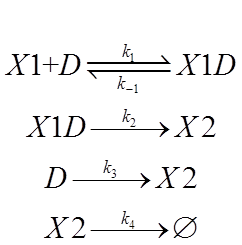
The symbol declaration is:
X1:tTA protein
D: the TRE promoter
X1D:the tTA-TRE complex
X2: the protein of interest
And we assigned each process with a reaction rate constant.
The first process is about binding and dissociation of molecules and is a fast reaction. Time unit for that is second. Since EF1-αis a constitutive promoter, and we define the initial state as when we remove the Dox from medium, we can regard the concentration of X1, or tTA protein, as a given value, determined by intensity of EF1-α. Reaction rate constant k1,k-1 are affected by Dox. In the tolerable range descried in part3, the more Dox we apply to D, the smaller value of k1 for the positive direction and the greater value of k-1 for the negative direction.
In the second and third process, k2 and k3 are affected by what kind of TRE promoter we use. There are several available TRE promoters, with which we can assemble different version of Tet-off system. These promoters differ in leaky expression and switching performance.
MiRNA-mediated mRNA degradation lead to a decrease in X2 production, which can be thought as identical with natural degradation of X2, the protein of interest. So K4 will be affected by the knockdown efficiency of miRNA binding site. We have constructed several binding sites to fine tune this process.
2.2 solutions and implication
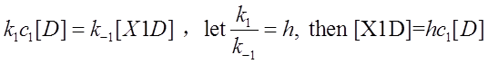
According the analysis, we then wrote down the ODEs:
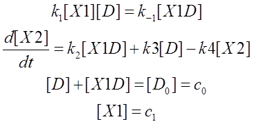
Here [D0] is the initial concentration of promoter Pcmv,c1 is the given concentration of X1 at the beginning. Next we will do some algebra to simplify the equations and solve the differential equations.
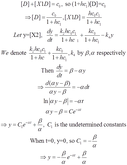
We use Mathematica’s Dynamic Interactive Function Manipulation to control the variation of the parameters α,β, and thus get curves with different dynamics and steady state.
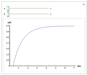
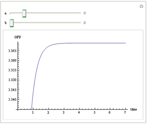
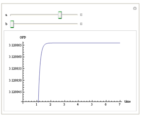
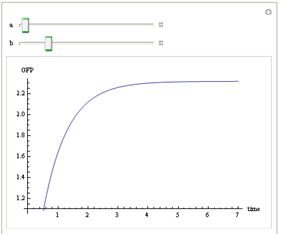
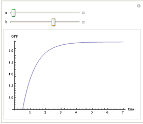
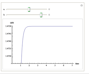
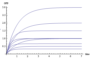
Figure 1. Different values of α,βgenerate curves with different dynamics and steady state.
As analyzed in 2.1, choosing different candidates with variant characteristic will affect the parameters in the chemical reactions, and change values of α and β. We’ve got 4 tet-off systems, a series of miR122 binding sites and experimental characterize them. And also we have two EF1-α promoters with different enhancers(not mentioned in Result section). This implicate that we can assemble different circuits and fine-tune the dynamics and steady state. We believe that this is important to practical engineering, just as basic logic is to conceptual designing.
3. Dosage effect of DOX in turning off the Tet-off system
DOX ,as is discussed above, hinders the binding of tTA to pTRE in Tet-Off system and knockdown expression of suicide gene. In our experiment, we employ fluorescence technique to manifest the amount of protein product by detecting the strength of the fluorescence.

Table 1. Stimulating data of GFP-Dox

Figure 4. GFP-Dox line chart
Our task is to find the proper curve to fit the sample data. First of all we plot the scatter diagram, and according to its tendency, we use type curve to fit the relation of GFP-DOX. We use MATLAB to aid our fitting, i.e. to determine the parameter a, b and k.

%expun.m
function y=expun(s,t) %coefficient and variable
y=s(1)+s(2)*exp(-s(3)*t)
%curvefit.m
treal=[0 0.125 0.25 0.5 1 2]; %experimental data
yreal=[25 13 10 8 6 5.7];
s0=[0.2 0.05 0.05]; %iteration initial value
sfit=lsqcurvefit('expun',s0,treal,yreal); %least square curve fit
f=expun(sfit,treal);
disp(sfit);
The result :

Figure 5. Running result
So a=6.4147,b=18.3999,k=7.3173.
Then we program the diagram file GFP-DOX.m
%GFP-DOX curve
treal=[0 0.125 0.25 0.5 1 2]; %experimental data
yreal=[25 13 10 8 6 5.7];
t=0:0.1:2.5;
a=6.4147;b=18.3999;k=7.3173;
y=a+b*exp(-k*t);
plot(treal,yreal,'rx',t,y,'g');
xlabel('Dosage of DOX');
ylabel('GFP');

Figure 6. GFP-Dox curve
As is shown in the figure above, we can conclude that the amount of GFP tend to be steadily over 1.5 ug, the higher concentration of DOX we set, the lower GFP we expect. However, under the real experimental conditions, over 2.2 ug DOX will lead to the undesired necrosis of the cells. This is a trial-experiment which proved that such a balance point for good turning- off effect and cell tolerance does exist in a certain interval concentration. More accurate experiment should be conducted on stable-transfected iPSCs to find the best cultivating condition.
4. Knockdown efficiency interpolation
According to the experimental data, here we use interpolation technique to find the relationship between miRNA-122 concentration, the number of miR122 target sites and cell knockdown efficiency, which leads to a function with two variables. The knockdown efficiency is represented by GFP expression level which is actually the ratio of the amount of GFP and that of the parameter GAPDH. The knockdown efficiency then is


Figure 7. Two target sites, gradient miRNA concentration

Table 2. Experimental data of 2 target sites, gradient miRNA concentration

Table 3. Experimental data of 0.75ug miRNA plasmid with gradient target sites
We use the data above to do the interpolation. We use the griddata function to implement the interpolation.
MATLAB codes:
clear
miRNA=[0 0.025 0.05 0.1 0.25 0.75 0.75 0.75];
site=[2 2 2 2 2 1 2 4];
KD=[0 29 43 55 64 55 39 32];
cx=0:0.01:0.75;
cy=0:0.05:4;
cz=griddata(miRNA,site,KD,cx,cy','cubic');
meshz(cx,cy,cz),rotate3d
%shading flat
xlabel('miRNA(plasmid ug)'),ylabel('Target Site'),zlabel('knockdown efficiency(%)');

Figure 8. Knockdown efficiency-mRNA-target site surface chart
5. The excursion of little mathematician--Data analysis of the FACS data
When our project was proceeding, we found out an interesting problem, that is, how to calculate the killing efficiency of each suicide gene? And this quantity is also an important part of our modeling. Trying to solve this problem,one of our mathematician, young Yang ZiYi, excursed a little bit from modeling to data analysis. And he analyzed our data of FACS of our transient transfection experiment of Hep G2.
One important point in mathematical analysis about the complicated biological system is, not to draw arbitrary assumption, arbitrary assumption just lead to disaster. Another important point is not to draw complicated assumption, which is hard to calculate. Base on these rules, Young ZiYi draw some simple and reasonable assumptions:
1. The initial condition of each parallel well is the same, that means, every well before transient transfection should have the same cell density, and the cells' state should be approximately the same.
2. In the GFP control group, the cells should be regarded as the same, whether they are transfected with GFP or not, since GFP do not harm the cells. But lipo-2000 will harm the cells, and may have some long term effect. So the GFP control group would be relatively weaker compare to negative control, which without any transfection manipulation;
3. The cells transfected with GFP should have an innate death rate r1 after 3 days cultivation. Besides, the ratio of “the initial number of cells” to “the number of cells harvested via FACS after 3 days” Should be the same, since if you sample any part of the wells you will observe the same distribution of cells, this means the cell experiment is scalable. Hence, we can define a special “state” to represent GFP cells in certain well, (r1,n1), n1 is the number of the cells we harvest in 30s, depends on r1 and the initial cell number.
4. In the well we transfect suicide genes, the cells which are transfected with suicide gene will be different from the cells which are not, due to the killing effect of suicide gene, and the cells without transfection will be at the same condition as GFP control and have the same r1. Cells transfected with suicide gene will have a different r2, we denote this part of cells by (r2,n2). If the transfection efficiency is a, then for any initial cell number N0, there will be N0×a cells transfected with suicide gene, the remaining N0×(1-a)are not. Here "a" in an unknown factor.
Then Young ZiYi built a model:
In the wells that had been tranfected with suicide genes, the final observed “state” (X, C) of the cells is an combination of two kinds of cells, one kind with state (r1,n1), the other kind with state (r2,n2). The effect of these two kinds will be summed up together. Then we can write down a equation:

Because we can not easily get the transfection efficiency, we select a reasonable range from experience:[30%,60%], and solve the equation with the data from FACS, and get the following results:
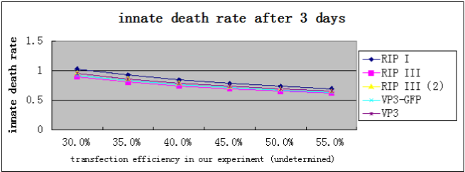
It turns out that, the death rate of cells transfected with suicide gene will be greater than 60%, significantly higher than normal cells and GFP control cells(29.07%, according to our data).
Then, We pick up one suicide gene, VP3, and take an “a” value 35% which we believe is fairly closed to the real tranfection efficiency, solve the equation and get the result r2 and n2. And then, we substitute the calculated r2 and n2 to the left side of the equation, and raise the value of “ a” to predict what the death rate and the “number per 30 seconds” would be when the transfection efficiency is raised. The result is shown in a chart below
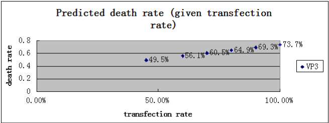

That makes our model become a real theory, because it predicts something that can be disproved. In the following day, we will try to raise our transfection efficiency, and try to comparing the result with the prediction.
And, let’s wait for the result.
6. Multi-compartment model
6.1 Analysis of the problem
We firstly focus on factors that regulate the performance of the whole pathway. Protein tTA expressed by a EF1α promoter binds to the promoter pTRE to drive the transcription of target gene( in this case, eGFP or suicide gene) while Dox acts as a co-repressor prohibiting the transcription. MiR122 isa downstream part in the pathway after transcription of target mRNA, and mediated degradation of the mRNA, thus rescue the cell or knockdown its GFP expression. However, the miR122 level in iPSC was low and insufficient to exert obvious effect on the expression.
Apart from Dox concentration,we also monitored other parameters, including cell number after the stable infection and number of cell that survived the Suicide Gene. Moreover, we also kept track of fluoresence intensity of the control group who has been transfected with GFP, which can be employed to indicate the GOI expression level driven by Tet-Off system.
In pratical, we planned to monitor the cell group scale every 5 hours and technically, we counted the total clone area instead of cell number.
6.2 Symbols declaration and assumption
X1: initial number of iPS cells with Suicide Gene
X2: number of the iPS cells whose TRE have been combined with tTA
X3: number of iPS cells which have died from expressing Suicide Gene
k1: converting rate of the number of cells from phase X1 to phase X2
k2: converting rate of the number of cells from phase X2 to phase X3
The unit of ki(i=1,2) is hour-1.We measured it by dividing the absolute value of the cell number difference between former phase and latter phase, with the time period length.
Two cases are taken into account. In case (a), self-renewal and replication of cels are ingored while in case (b), we take that into consideration. To further simplify the model, we also assumed that every single cell in phase X1 turns into n1 state before phase X2, and every single cell in phase X2 turns into n2 state before phase X3. We simulated the kinetic process of gene expression and assumed an even distribution of cell content in the medium,after which the phase can be regarded as a compartment.
6.3 Solution
For each compartment, we construct unsteady state equilibrium equation, hence we obtain the ordinary equations

For case (b), we just need to modify the scalar coefficients of the equations above, and we obtain


Figure 1. dynamic process
We are going to solve X1(t), X2(t),X3(t), then we will plot the time course curve.
The initial conditions of the differential equations are as follows:
X1(0)= 5000 cells, X2(0)=0 cell, X3(0)=0 cell
k1=1day-1,k2=1 day-1
As for case b, the cell replicates every 26 hours, to simplify we consider one cell turns into 2 cells before next phase. Therefore, n1=n2=2.
Source code
%igem_test1.m-Solution of the IPS cell differentiation model
%using MATLAB function ode45.m to integrate the differential equations
%that are contained in the file cell_diff_eq.m
clc; clear all;
%set the initial conditions, constants and time span
xzero=[5000,0,0];tmax=4;
k1=1; k2=1;
tspan=0:0.1: tmax;
N=3;
%Integrate the equations
[t X]=ode45(@cell_diff_eq,tspan,xzero,[ ],k1,k2);
last=X(length(X),N);
%Plot time curve
plot(t,X(:,1),'-',t, X(:,2),'-',t, X(:,3),'-.');
legend('X1','X2','X3');
xlabel('time,days');
ylabel('number of cells');
function dx= cell_diff_eq(t,x,k1,k2)
%cell expression kinetic procedure
dx=[-k1*x(1); k1*x(1)-k2*x(2); k2*x(2); ];

Figure 2. The result of case (a)

Figure 3. The result of case (b) 7.reference
[1] Systems biology in practice concepts, implementation and application / (德) E. Klipp等著 ; 主译:贺福初, 杨 芃原, 朱云平 ,上海 : 复旦大学出版社, 2007
[2]Numerical methods in biomedical engineering / (美) Stanley M. Dunn, Alkis Constantinides, Prabhas V. Moghe著 ; 封洲燕译,北京 : 机械工业出版社, 2009
[3]miRNA regulatory circuits in ES cells differentiation: chemical kinetics modeling approach , Luo Z, Xu X, Gu P, Lonard D, Gunaratne PH, et al. (2011)
[4]kinetic signatures of microRNA modes of action, N Morozova, A Zinovyev, N Nonne, LL Pritchard - RNA, 2012
[5]On the inhibition of the mitochondrial inner membrane anion uniporter by cationic amphiphiles and other drugs. Beavis AD,J Biol Chem. 1989 Jan 25;264(3):1508-15.
Sun Yat-Sen University, Guangzhou, China
Address: 135# Xingang Rd.(W.), Haizhu Guangzhou, P.R.China