"
"
Team:UCSF/Modeling2
From 2013.igem.org
| Line 84: | Line 84: | ||
| - | + | <div id="description" style = "width:950px; height:95px" align="justify"> | |
| - | + | ||
| - | + | ||
| - | + | ||
| - | + | ||
| - | + | ||
| - | + | ||
| - | + | ||
| - | + | ||
| - | + | ||
| - | + | ||
| - | + | ||
| - | <div id="description" style = "width:950px; height: | + | |
| - | + | ||
| - | + | ||
| - | + | ||
| - | + | ||
<font face="calibri" size = "4"> | <font face="calibri" size = "4"> | ||
| - | + | In order to simulate the RFP levels, we need to model the population dynamics of our system. Thus these equations have been to model the three strains present in this system: | |
| - | + | ||
| - | + | ||
| - | + | ||
| - | + | ||
| - | + | ||
| - | + | ||
| - | + | ||
| - | + | ||
</div> | </div> | ||
| - | + | <div id="description" align="justify" style = "width:950px; height:40px"> | |
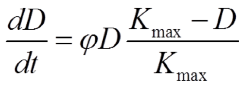
| - | <div id="description" style = "width:950px; height: | + | <p><font face="calibri" size = "4">Engineered Donor Cell levels:</font> |
| - | <font face="calibri" size = "4"> | + | |
| - | + | ||
</div> | </div> | ||
| - | + | <div id="photos"> | |
| + | <center><img style="height:60px;margin-top:10px"; padding:0;" | ||
| + | src="https://static.igem.org/mediawiki/2013/8/86/Conj_EQ2_UCSF.png"> </center></div> | ||
<div id="photos"> | <div id="photos"> | ||
Revision as of 01:57, 29 October 2013


The primary goal of the modeling portion for the CRISPRi conjugation project is to create a model that will help us identify the behavior of our transferable targeting system and identify critical parameters, given our assumptions. We used this model to check whether our CRISPRi conjugation system would have the desired behavior under biologically relevant parameters.
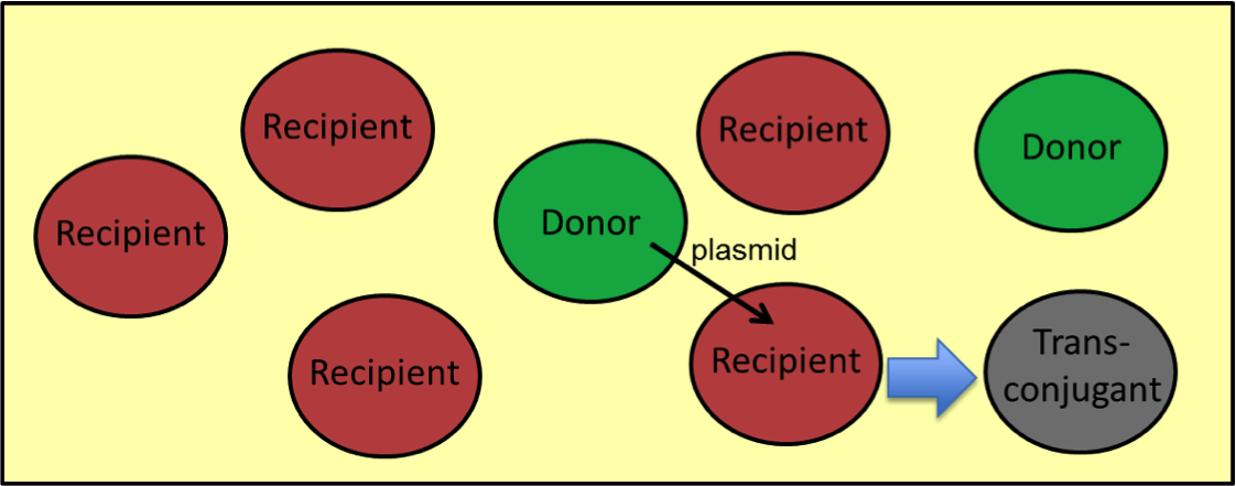
This system is designed to be transferred from cell to cell, targeting a specific gene of interest within the community. We model the activity of three strains of E. coli, an engineered donor strain containing a conjugative plasmid with genes coding for dCas9 and a gRNA, a recipient strain containing the RFP gene (target gene) in its genome, and upon successful conjugation, a transconjugate strain that no longer expresses RFP as well as the community's total RFP concentration.
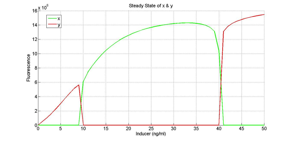
Our objective is to simulate this community over time to see if our engineered system causes RFP levels to decrease.
ASSUMPTIONS: While creating the model for our system, we made four assumptions in order to simplify some of the aspects of the model. Many similar assumptions have been made in the literature.
1) RFP, dCas9, and gRNA are produced and degraded at a constant rate;
2) conjugation rate is linearly dependent on the concentration of donor and recipient cells (mass action);
3) CRISPR expression efficiency in a cell is 100%;
4) The growth rates of the three strains are equal.
EQUATIONS
Given these assumptions we have the following equations for the system:
Change in RFP levels over time:
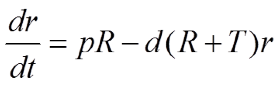
p – RFP production rate in a single cell
d – RFP degradation rate in a single cell
And the variables in this equation are:
r – concentration of RFP
t – time
R – number of recipient cells
T – number of transconjugant cells
Engineered Donor Cell levels:
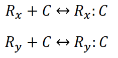
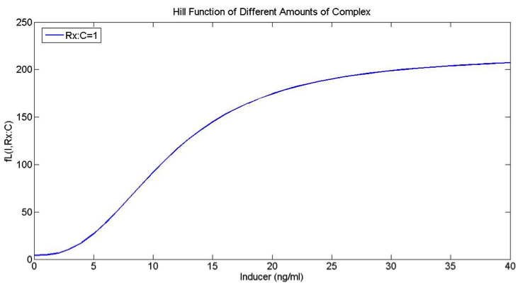
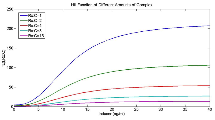
Given these chemical reactions, we can write the following equations for the gRNA/dCas9 Complex:
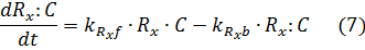
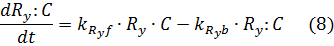
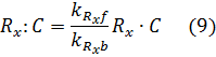
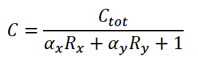
Under that assumption (setting equations (7) and (8) to zero – known as the quasi steady state assumption), we can solve for the complex in terms of the unbound repressor concentrations:
Where the amount of dCas9 available in the system is given by:


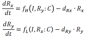
The equations for the gRNAs depend on the amount of the gRNAs that is produced, the degradation rate, and also the rate at which the gRNA complexes with dCas9. With the quasi-steady state assumption, the terms for complexing with dCAS9 drop out and the final equations for the gRNAs are similar to equations (1) and (2) for the fluorescent proteins:
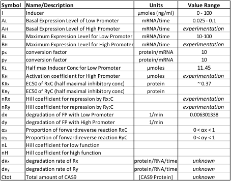
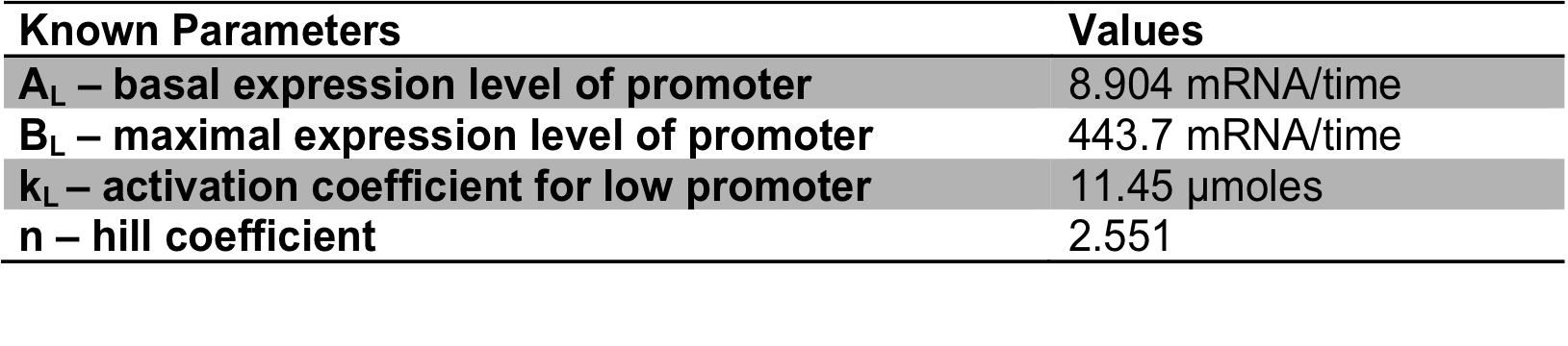
PARAMETERS
This model has many parameters, so in order for it to be more useful, we need to reduce the number of parameters that are undetermined. To accomplish this, we gathered some values from literature and also did experiments to find other parameters (Table1).
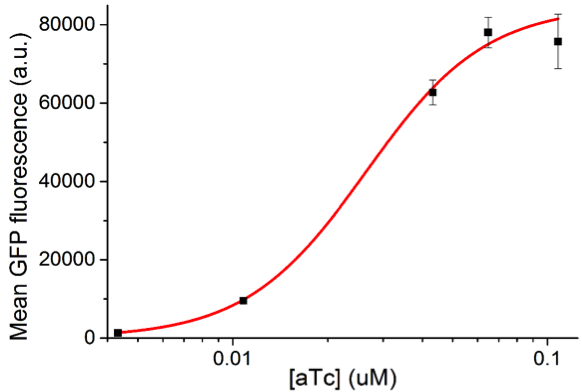
How does the model look with our actual “low” and “high” promoters?
If the only change in the low and high functions (FH and FL) is the K values (which determine the sensitivity of the promoters), then we don’t get our desired behavior. However, there are other parameters that might give us the desired behavior for the low and high promoters.
If we set BL to 443.7 and BH to 443.7*1.25, and if we set the half max values to kL = 11.45 and kH=17, the promoters have the following profile:
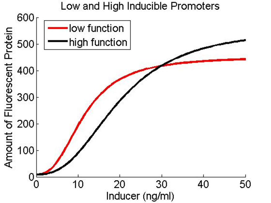
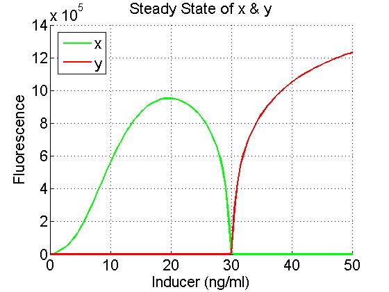
How does the system change when the hill coefficient is manipulated? In this first plot, the hill coefficients for both the low and the high function are the same number: 2.551. This number is the one we determined from our experimental data.
nL = 2.551
nH = 2.551
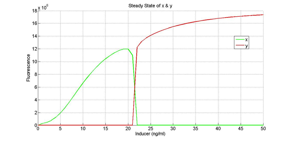
nL = 2.551
nH = 1.551