 "
"
Team:Valencia Biocampus/Demonstration/Diffusion3
From 2013.igem.org
(→Proof of a Group Behavior Diffusion Model from a Random Walk Model) |
Beta3designs (Talk | contribs) (→Proof of a Group Behavior Diffusion Model from a Random Walk Model) |
||
| (31 intermediate revisions not shown) | |||
| Line 11: | Line 11: | ||
== Proof of a Group Behavior Diffusion Model from a Random Walk Model == | == Proof of a Group Behavior Diffusion Model from a Random Walk Model == | ||
| - | + | To prove that, we will make the assumption that the worm only moves in one dimension ($x$) without loss of generality. | |
<br/> | <br/> | ||
<br/> | <br/> | ||
| Line 57: | Line 57: | ||
<br/> | <br/> | ||
<br/> | <br/> | ||
| - | $$ P(x,t)\;=\;\frac{1}{\sqrt{4 | + | $$ P(x,t)\;=\;\frac{1}{\sqrt{4 \pi D t}}\;e^{-\left(x - v t\right)^2/\left(4 D t\right)}$$ |
| - | + | ||
</li> | </li> | ||
</ul> | </ul> | ||
</html> | </html> | ||
| - | |||
| - | |||
| - | |||
| - | |||
| - | |||
| - | |||
| - | |||
| - | |||
| - | |||
| - | |||
| - | |||
| - | |||
| - | |||
| - | |||
| - | |||
| - | |||
| - | |||
| - | |||
| - | |||
| - | |||
| - | |||
| - | |||
| - | |||
<br/> | <br/> | ||
<div style="text-align:center;"> | <div style="text-align:center;"> | ||
<html> | <html> | ||
| - | <a href=""><img src="https://static.igem.org/mediawiki/2013/ | + | <a href=""><img src="https://static.igem.org/mediawiki/2013/a/a7/Diffus.png" width="700" height="300" alt="Allowed directions"/></a> |
<br/> | <br/> | ||
| - | <span style="font-size:10px"> | + | <span style="font-size:10px">Plots of $\;P(x,t)\;$ for different $\;v\;$, and different time instants: left, $\;D$ = $1\;$ and $\;v$ = $1\;$; right, $\;D$ = $1\;$ and $\;v$ = $2\;$</span> |
</html> | </html> | ||
</div> | </div> | ||
| Line 96: | Line 72: | ||
<br/> | <br/> | ||
<br/> | <br/> | ||
| - | |||
<br/> | <br/> | ||
| - | + | ||
| - | + | ||
| - | + | ||
| - | + | ||
| - | + | ||
| - | + | ||
| - | + | ||
| - | + | ||
| - | + | ||
| - | + | ||
| - | + | ||
| - | + | ||
| - | + | ||
| - | + | ||
| - | + | ||
| - | + | ||
| - | + | ||
| - | + | ||
| - | + | ||
| - | + | ||
| - | + | ||
| - | + | ||
| - | + | ||
| - | + | ||
<br/> | <br/> | ||
----- | ----- | ||
Latest revision as of 08:53, 4 October 2013

Proof of a Group Behavior Diffusion Model from a Random Walk Model
To prove that, we will make the assumption that the worm only moves in one dimension ($x$) without loss of generality.
At each time step $\;q\;$ it either moves a distance $\;h\;$ to the left with probability $\;l\;$, a distance $\;h\;$ to the right with probability $\;r\;$, or stays in the same position with probability $\;1−r−l\;$ (the isotropic random walk has $\;r\;=\;l\;=\;1/2$, so it cannot rest motionless). We also define the probability that a worm is at a position $\;x\;$ at time $\;t\;$ by $\;P(x,t)\;$. One time step earlier, at time $\;t − q\;$, the walker must have been at position $\;x − δ\;$ and then moved to the right, or at position $\;x + δ\;$ and then moved to the
left, or at position $\;x\;$ and then not moved at all. Thus:
$$ P(x,t)\;=\;P(x,t-q)\;\left(1 - l - q\right) + P(x-h,t-q)\;r + P(x+h,t-q)\;l $$
Assuming that $\;q\;$ and $\;h\;$ are so small, that are negligible compared to $\;t\;$ and $\;x\;$ respectively, we can expand de function as a Taylor series, around $\;t\;$ and $\;x\;$. Notice that higher terms than $\;q^2\;$ and than $\;h^3\;$ have been included in $\;O(q^2)\;$ and $\;O(h^3)\;$, respectively:
$$ P\;=\;\left(P - q\;\frac{\partial P}{\partial t}\right)\;\left(1 - l - r\right) + \left(P - q\;\frac{\partial P}{\partial t} - h\;\frac{\partial P}{\partial x} + \frac{h^2}{2}\;\frac{\partial^2 P}{\partial x^2}\right)\;r + \left(P - q\;\frac{\partial P}{\partial t} + h\;\frac{\partial P}{\partial x} + \frac{h^2}{2}\;\frac{\partial^2 P}{\partial x^2}\right)\;l + O(h^3) + O(q^2)$$
Rearranging this gives:
$$ \frac{\partial P}{\partial t}\;=\;\frac{\alpha\;h^2}{2\;q}\;\frac{\partial^2 P}{\partial x^2} - \frac{\beta\;h}{q}\;\frac{\partial P}{\partial x} + O(h^3) + O(q^2)$$
Where $\;\alpha\;=\;r + l\;$ and $\;\beta\;=\;r - l\;$. We now let $\;h,\;q,\;\beta\;\rightarrow\;0\;$ in such a way that the following
limits are finite:
$$ D\;=\;\alpha\;\lim\limits_{h,\;q,\;\beta\rightarrow 0}\frac{h^2}{2\;q} $$
$$ v\;=\;\lim\limits_{h,\;q,\;\beta\rightarrow 0}\frac{h\;\beta}{q} $$
So we can neglect $\;O(h^3)\;$ and $\;O(q^2)\;$, resting:
$$ \frac{\partial P}{\partial t}\;=\;D\;\frac{\partial^2 P}{\partial x^2} - v\;\frac{\partial P}{\partial x} $$
Considerations:
-
If we set $\;r\;=\;l\;=\;1/2\;$ as in the isotropic random walk, then $\;\beta\;=\;0\;$, so $\;u\;=\;0\;$, giving as a result the non-biased Diffusion Equation:
$$ \frac{\partial P}{\partial t}\;=\;D\;\frac{\partial^2 P}{\partial x^2}$$
-
In this case, $\;v\;$ is constant for all the space, not as in the case that concerns us, where $\;v\;$ depends on the gradient of the attractant, normally distributed (with Gaussian Distributions) in the space of interest. So, with $\;v\;$ constant, it is possible to obtain an analytical solution, given by Montroll & Shlesinger (1984), with initial condition $\;P(x,0)\;=\;\delta(x)\;$, that is:
$$ P(x,t)\;=\;\frac{1}{\sqrt{4 \pi D t}}\;e^{-\left(x - v t\right)^2/\left(4 D t\right)}$$
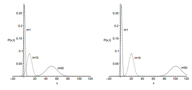
Plots of $\;P(x,t)\;$ for different $\;v\;$, and different time instants: left, $\;D$ = $1\;$ and $\;v$ = $1\;$; right, $\;D$ = $1\;$ and $\;v$ = $2\;$
Okopinska A. (2002) Fokker-Planck equation for bistable potential in the optimized expansion. Physical review E, Volume 65, 062101