 "
"
Team:Valencia Biocampus/Modeling
From 2013.igem.org

Modeling
The main goal of our modeling project is to accurately predict the behavior of our system in several issues, from the mounting of bacteria on C. elegans to the performance of our worms reaching the place of interest. In order to do that, we use several modeling techniques.
The movement of C. elegans in the presence of a chemoattractant in order to carry our bacteria to that source is the main issue of our project, so we consider modeling this aspect and employing it as scaffold for the whole modeling project. Several layers show up that it must be modeled in different ways. In our approach, we mathematically describe each layer, from the simplest to the most complex, integrating each one.
The workflow in the C. elegans movement is the following:
| Single Worm Behavior | Single Worm Chemotaxis | Group Behavior | System performance | ||
|---|---|---|---|---|---|
| Considerations | Chemoattractant | ||||
| Bacteria | |||||
| Modeling approach | Random Walk | Biased Random Walk | Partial Differential Equations | Ordinary Differential Equations | |
The model is improved adding the data obtained from the experiments in order to achieve a holistic model which can predict the distribution of our worms, the kinetics of the present bacteria and the concentration of the substrate in each moment.
Biobricks modeling
In this section, PHA production is modeled.
PHA production
By extracting data from fermentation assays we obtained a good simple linear regression by means of the least squares method between the dry weight of the microorganismos (Pseudomona Putida) and the PHA weight produced, the relationship we obtained is as follows:
$$ PHA = 0.2022 \cdot CellDryWeight $$
Where $ PHA $ and $ CellDryWeight $ are in grams ($ g $). The average for the prediction error is $\mu = 0.2008$ and the variance $\sigma^2 = 1.9005$. The coefficient of determination is $R^2 = 0.9374 (93.74\%)$.
The equation with all the data is represented below:

The red dots near the origin correspond to a batch fermented in a flask, the blue dots correspond to an assay with two fedbatches in a fermenter of 2 liters. The black line is the linear regression line obtained by the least squares' method.
C. elegans behavior
In order to understand the system as a whole, we started with the simplest case, so our first study is based on the behavior of a single worm, initially in the absence of chemoattractant and later adding it.
Our first approach consists in the study of a single worm in a surface without chemoattractant, under this condition it is observed that a C. elegans moves randomly, this is defined as a Random Walk.
Random Walk is the mathematical formalization of a trajectory that consists of taking successive random steps. We ran several simulations in Scilab and C++, in order to represent a single C. elegans moving this way in the absence of attractants.
Random walks are used to describe the trajectories of many motile animals and microorganisms. They are useful for both qualitative and quantitative descriptions of the behavior of such creatures. In our case a single C. elegans was simulated as a point: $(x_t, y_t)$
At each instant $t$ in the simulation, step length $l_t$ and direction $\theta_t$ the equations are the following:
$$l_t = \Delta t\;\nu_t$$
$$\theta_t = \theta_{t-1} + \Delta t \left(\frac{d\theta_t}{dt} + \delta\right) $$
Where $\Delta t$ is the duration of the time step, $\nu_t$ is the instantaneous speed, $\frac{d\theta_t}{dt}$ $(= \dot{\theta_t})$ is the instantaneous turning rate (using the convention that $\frac{d\theta_t}{dt}$$ > 0$ is a right turn and $\frac{d\theta_t}{dt}$$ < 0$ is a left turn) and $\delta$ is the turning bias.
The values of these variables were taken randomly from different gaussian distributions, that we identified by sampling but also obtained from some papers:
$\nu_t$: normal distribution with $\sigma = 0.0152\;cm/s$ and $\mu = 0.00702\;cm/s$
$\dot{\theta_t}$: normal distribution with $\sigma = 0.0150273\;rad/s$ and $\mu = 0.6789331\;rad/s$
$\delta$: normal distribution with $\sigma = 0.0076969\;rad/s$ and $\mu = 0.0370010\;rad/s$
Simulations were performed in Scilab and C++, proceeding as described in (Pierce-Shimomura et al., 1999). We contacted the authors but they could not provide us with the code, so we developed our own script based on the article, obtaining similar results:
You can also simulate C.elegans random walk in our Simuelegans online application
Simulated with our own software SimuElegans.
Please note that the actual movements of C. elegans are much slower and thus the simulation in this video is accelerated for convenience.
In these simulations we considered $\Delta t = 1\;s$, but actually we simulated it every $0.01\;s$, so its $\frac{1\;s}{0.01\;s} = 100$ times accelerated.
Chemotaxis of a single worm
However, we are interested in the movement of the nematode in a gradient of chemoattractant.
Studies revealed that the behavior of E. coli during chemotaxis is remarkably similar to the behavior of a single C. elegans in the presence of a chemotactic source (Bargmann, 2006), a mechanism called the pirouette model in C. elegans (Pierce-Shimomura et al., 1999) and the biased random walk in bacteria (Berg, 1993; Berg, 1975). The basis of these models is a strategy that uses a short-term memory of attractant concentration to decide whether to maintain the current direction of movement or to change to a new one.
Following this model, we defined the turning rate as a function of $\frac{\partial [C]}{\partial t}$. Where $[C]$ is the concentration ($[\;]$) of chemoattracant ($C$). Simulations were performed as expected, showing a bias in the random walk:
You can also simulate C.elegans chemotaxis in our Simuelegans online application
Simulated with our own software SimuElegans.
Chemotaxis of a single worm consuming attractant
As a last step of the study of a single worm, we decided to modelize the most realistic behavior. This behavior happens when, in addition to moving randomly but biased toward the gradient of chemoattractant, we consider the fact that it is constantly consuming its “food”, so these gradients will not be any more constants in time.
In order to implement this model, we realized that was impossible to study still considering the space as an attractant function, cause it changes its shape in every time step, and it made simulations really slow (maybe, days of computation). So, we meshed the space, and gave every point a different weight, depending on time: that was the starting of the matrix and approximated (numerical) calculations. What we obtained was close to have relevant impacts in the course of our project, because we could interfere in the C. elegans path, and not only in its final position, making it moving from one source of chemoattractant to another:
Simulated using Scilab
Note that this simulation has been speeded 600%.
Moreover, these numerical methods opened our eyes to study their movement as a whole, with partial differential equations.
Bargmann CI (2006) Chemosensation in C. elegans. Wormbook
Berg HC (1993) Random walks in biology. Princeton, NJ: Princeton UP.
Pierce-Shimomura JT, Morse TM, Lockery SR (1999) The Fundamental Role of Pirouettes in C. elegans Chemotaxis. The journal of Neuroscience, 19(21):9557-9569
Group behavior
In practice, a single C. elegans is not employed to perform the task but a group of worms. In this case, the random walk equations obtained for a single worm behavior can be transformed into partial differential equations (PDEs), using Taylor series, to depict the distribution of the population, as the ones describing a diffusion process (![]() Click here for a mathematical proof of one dimensional diffusion process using PDEs from random walk)
Click here for a mathematical proof of one dimensional diffusion process using PDEs from random walk)
However, in our case we face a diffusion system with drift, in which the last term arises from the biased movement of C. elegans. To obtain a PDE that reflects this behavior, we employed difference equations also using Taylor series and apropiate limits (![]() Click here for a mathematical proof of two dimensional biased diffusion process (C. elegans chemotaxis behavior) using PDEs from biased random walk)
Click here for a mathematical proof of two dimensional biased diffusion process (C. elegans chemotaxis behavior) using PDEs from biased random walk)
The equation is the following:
$$\frac{\partial [C]}{\partial t} = D\;\nabla^2[C] - \nabla\cdot(\underline{\nu}\;[C]) $$
Once obtanied the equation that governs our system, we proceed to study if it works correctly for our purpose. However, analytical solutions for this equation are known for few ideal cases. For example, for a monodimensional bistable potential the stationary state is the following (Okopinska, 2002):
$$ P_{ss}=\mathscr{N}^{-1} e^{\left(-V(x)/D\right)}$$ where $ \mathscr{N} $ is the normalization constant.

As seen, our system, can theoretically work as expected, depending on the shape of the chemoattractant only. This is a great result because it shows our worms are capable of reaching each region.
Finally, our final goal in this section is predicting temporal and spatial behaviour in two dimensions for non-ideal problems. In this case, numerical methods is the only way to solve the system.
For the 2-dimensional case, $[C] = [C(x, y, t)]$ is the concentration of C. elegans at a given instant $t$ and at a given point $(x, y)$, $D$ is the diffusion coefficient and $\overrightarrow{\nu}$ is the attraction field for the C. elegans, which basically stands for its velocity. This expression naturally expands to: $$\frac{\partial [C]}{\partial t} = D \; \left(\frac{\partial^2 [C]}{\partial x^2} + \frac{\partial^2 [C]}{\partial y^2}\right) - \left(\frac{\partial\nu_x}{dx}[C] + \nu_x\frac{\partial [C]}{\partial x} + \frac{\partial\nu_y}{dy}[C] + \nu_y\frac{\partial [C]}{\partial y}\right) $$
We first started by building up an explicit finite difference method, this is numerically fast but it is prone to instabilities in the solutions. Therefore, we decided to develop a Crank-Nicolson method which is unconditionally stable, thus being suitable to carry out parameter identification of a model. Nevertheless, it has the drawback of being numerically more intensive, because a set of algebraic equations must be solved in each iteration (![]() Click here for a mathematical explanation of the Crank-Nicolson method).
Click here for a mathematical explanation of the Crank-Nicolson method).
Now, we can predict the behavior of a set of worms in presence of a chemoatractant. One must have into account that the system may behave differently depending on some variables, for example, the diffusion coefficient $D$, a constant $k$ that determines the weight that the drift variable $\nu$ has and the time constants for the chemoattractant diffusion $t_1$ and $t_2$, where $t_1$ is the elapsed time since a first chemoattractant drop is put into the petri plate, $t_2$ stands for the elapsed time since a second drop of chemoattractant is put into the petri plate until a C.elegans initial distribution is added, the diffusion of chemoattractants is then assumed to be negligible for simplicity reasons. According to these parameters, we performed a lot of simulations using SciLab, what they all have in common is the position of the four chemotactic sources. The simulations were performed by first varying only $t_1$ and $t_2$ for some given $D$ and $k$ ($D = 0.2$ & $k = 0.001$):
 $t_1$ = 5, $t_2$ = 6
 $t_1$ = 5, $t_2$ = 12
 $t_1$ = 10, $t_2$ = 12
 $t_1$ = 10, $t_2$ = 24
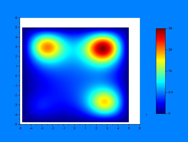 $t_1$ = 15, $t_2$ = 24
 $t_1$ = 15, $t_2$ = 48
It can be observed by ploting the drift field for each case, that the final distribution is mostly dependent on the mentioned drift field, which in fact is mostly dependent on $t_1$ and $t_2$. Here we present the drift fields for each case:
 $t_1$ = 5, $t_2$ = 6
 $t_1$ = 5, $t_2$ = 12
 $t_1$ = 10, $t_2$ = 12
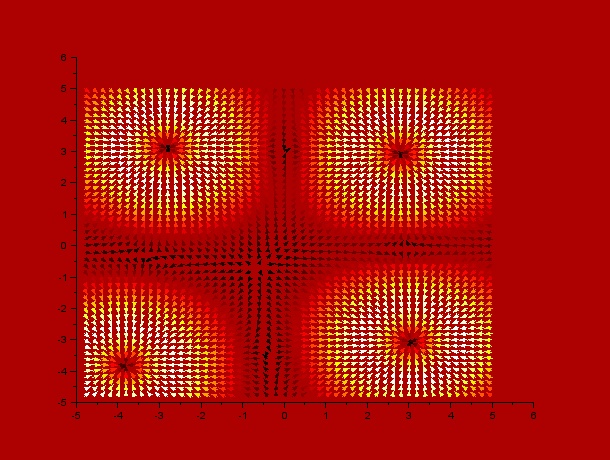 $t_1$ = 10, $t_2$ = 24
 $t_1$ = 15, $t_2$ = 24
 $t_1$ = 15, $t_2$ = 48
Qualitatively, it can be seen through these simulations that incrementing $t_1$ or $t_2$ disperses and smoothes the drift field which actually affects the final distribution of C.elegans by dispersing it.
Videos corresponding to each simulation can also be seen here:
And then by varying only $D$ and $k$ (separately, of course) for some given $t_1$ and $t_2$ ($t_1 = 10$ hours & $t_2 = 12$ hours):
 D = 0.05, k = 0.001, D/k = 50
 D = 0.1, k = 0.001, D/k = 100
 D = 0.2, k = 0.001, D/k = 200
 D = 0.05, k = 0.0005, D/k = 100
 D = 0.1, k = 0.0005, D/k = 200
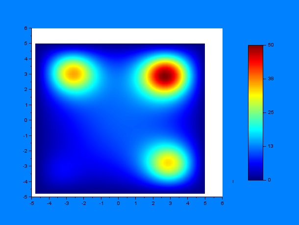 D = 0.2, k = 0.0005, D/k = 400
According to these results, qualitatively, higher values of $D$ or lower values of $k$ (and thus a greater $D/k$ relation) give a much more disperse distribution of C.elegans.
Videos corresponding to each simulation can be seen here:
We also did some simulations with different number of attractant sources, but as we consider they weren't so illustrative, we didn't make the studies with them. Here there are simulations with $1$, $2$ and $3$ sources, and parameters $D\;=\;0.2$, $k\;=\;0.001$, so $D/k\;=\;200$:
System performance
All this modeling part was made to track a set of worms in a given soil. This can be used to compare our system, a non-stirred solid bioreactor, with a conventional stirred liquid bioreactor. Simple ODEs for bacterial growth and substrate consumpton are used in a cualitative fashion to determinate the industrial applications.
Modelling this part is difficult because there are a lot of factors involved. Therefore, asumptions must be made. Our first approach is the study of the stationary state in both systems: In a stirred bioreactor, the concentration of both bacteria and substrate are constant whereas in a non-stirred one exists a determinated distribution. For the concentration distribution in the non-stirred bioreactor is gaussian and the bacteria distribution (consecuence of the attraction of C. elegans for the substrate) is given by the stationary state distribution for an one-dimensional case.
The pictures are graphical examples of both situations: Stirred case (left) and non-stirred (rigth). Substrate is shown in purple, bacteria in blue, and the relation between them in grey. The total concentration is the area below the curve. Values are arbitrary.
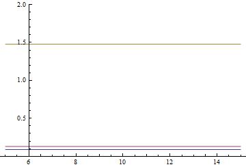

As can be seen, a higher bacteria/concentration ratio is achieved in our system than the conventional one. Anyone can appreaciate that the ratio tends to one, being lower than the conventional case ratio, but in that region the substrate concentration is nearly zero. So it is not interesting to study.
But one question arises: Is this significant? In fact, it is not. In both cases, the average ratio in the non-stirred case is the same as the stirred one. But it is not a drawback. It means that our system can perform the same as a conventional bioreactor but with the advantages of a higher concentration. Therefore, the production yield in higher.
In general, our system behaves as well as a conventional one for the stationary, linear, ideal case. Particular cases are not studied because they have to be analyzed independently. A complex model can be developed for each case to study its viability for its practical use, but it needs more time. Because of that, we made a cualitative study for the system. While time is a problem (stirring is faster than nematode crawling), higher yields and better suitability for several problems are important advantages of our system. Also, the combination of our model and the tracking device helps to determinate the final result.