Team:NCTU Formosa/modeling
From 2013.igem.org
Lsps9141105 (Talk | contribs) (→Ecolightuner Simulation) |
Darren820823 (Talk | contribs) (→Ecolightuner Simulation) |
||
| Line 53: | Line 53: | ||
===Ecolightuner Simulation=== | ===Ecolightuner Simulation=== | ||
<p>We have all the modeling of each single unit . Now, we want to combine each unit to make a stimulation to the E.colightuner. </p> | <p>We have all the modeling of each single unit . Now, we want to combine each unit to make a stimulation to the E.colightuner. </p> | ||
| - | [[File:Figure1_NCTU_Formosa.png|300px|center| | + | [[File:Figure1_NCTU_Formosa.png|300px|center|Figure 1. ]] |
<p>Figure 1 shows the essential constituent of our E. colightuner. To save our efforts experimenting with this essential engine of E. colightuner, we built a model beforehand to help us evaluate its practicability. Our model is consisted of three components A, B, C, and D</p> | <p>Figure 1 shows the essential constituent of our E. colightuner. To save our efforts experimenting with this essential engine of E. colightuner, we built a model beforehand to help us evaluate its practicability. Our model is consisted of three components A, B, C, and D</p> | ||
| + | [[File:Figure2_NCTU_Formosa.png|300px|center|Figure 2. ]] | ||
<p>Figure 2 is the overall picture of our component A. Notice that component A is built from similar biobricks as our E.colightuner. The only difference between the two is the promoters used. Both P<sub>red</sub> of E.colightuner are substituted with P<sub>cons</sub> in component A. With that said, by taking the difference in the strength between P<sub>red</sub> and P<sub>cons</sub>, into calculations, we would be able to model out E. colightuner with component A. Before that, however, we would have to first build a model for component A. </p> | <p>Figure 2 is the overall picture of our component A. Notice that component A is built from similar biobricks as our E.colightuner. The only difference between the two is the promoters used. Both P<sub>red</sub> of E.colightuner are substituted with P<sub>cons</sub> in component A. With that said, by taking the difference in the strength between P<sub>red</sub> and P<sub>cons</sub>, into calculations, we would be able to model out E. colightuner with component A. Before that, however, we would have to first build a model for component A. </p> | ||
| + | [[File:Figure3_NCTU_Formosa.png|300px|center|Figure 3.]] | ||
<P>To build a model for component A, we combined component B and C. As you can see in component B shown in Figure 3, it does not include P<sub>lux</sub> and luxR like component A. By assuming that when luxR is expressed, P<sub>lux</sub> would immediately reach its full strength, however, we can consider luxR and P<sub>lux</sub> pair as simply a Pcons,that is constitutively activated. From this perspective, component A and B are the same, except that component A is also effected by the translation efficiency of 37<sup>o</sup>C RBS. Component C in Figure 4 is the model for 37<sup>o</sup>C RBS. So by multiplying component C and component B, we would be able to obtain a model for component A.</p> | <P>To build a model for component A, we combined component B and C. As you can see in component B shown in Figure 3, it does not include P<sub>lux</sub> and luxR like component A. By assuming that when luxR is expressed, P<sub>lux</sub> would immediately reach its full strength, however, we can consider luxR and P<sub>lux</sub> pair as simply a Pcons,that is constitutively activated. From this perspective, component A and B are the same, except that component A is also effected by the translation efficiency of 37<sup>o</sup>C RBS. Component C in Figure 4 is the model for 37<sup>o</sup>C RBS. So by multiplying component C and component B, we would be able to obtain a model for component A.</p> | ||
[[File:NCTU_A_simulated-value.jpg]][[File:NCTU_A_experimental-value.jpg]][[File:NCTU_A_modified-value.jpg]] | [[File:NCTU_A_simulated-value.jpg]][[File:NCTU_A_experimental-value.jpg]][[File:NCTU_A_modified-value.jpg]] | ||
Revision as of 14:53, 28 October 2013
Modeling was our first step forward. When validated with our experimental data, modeling is also a verification of the accuracy of our experiments.
Contents |
MATLAB Introduction
MATLAB (matrix laboratory) is a numerical computing environment and fourth-generation programming language. It is developed by MathWorks, a company in United States. MATLAB allows matrix manipulations, plotting of functions and data, implementation of algorithms, creation of user interfaces, and interfacing with programs written in other languages, including C, C++, Java, and Fortran. Although MATLAB is intended primarily for numerical computing, an optional toolbox uses the MuPAD symbolic engine, allowing access to symbolic computing capabilities. An additional package, Simulink, adds graphical multi-domain simulation and Model-Based Design for dynamic and embedded systems.
ANFIS Introduction
Adaptive-Network-Based Fuzzy Inference System, in short ANFIS, is a power tool for constructing a set of fuzzy if-then rules to generate stipulated output and input pairs. Unlike system modeling using mathematical rules that lacks the ability to deal with ill-defined and uncertain system, ANFIS can transform human knowledge into rule base, and therefore, ANFIS can effectively tune membership functions, minimizing the output error.
Single Unit
Red Promoter
As shown in Figure 1, the red promoter is consisted of Pompc and Plac. By multiplying the experimental data of Pompc + RBS + mGFP and Plac + RBS + mGFP, we would be able to build a model for the red promoter. This model, however, wouldn't be so accurate. To solve this problem, we used this model to train the actual experimental data of the red promoter by using ANFIS. Figure 2 is the result of such a training. We obtained a curve between our model and the actual experimental data. This curve is the representation of the new model that has been trained and supported by the actually experimental data of Pred. This new model definitely contains a high degree of accuracy.
Lux Promoter
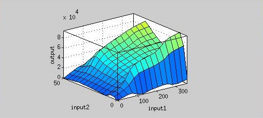
We did the following modeling based on the data obtained from Imperial 2007 iGEM team. The data notes the strength of Plux under different concentrations of AHL and different time frames.
Using ANFIS to train 76 sets of data and to test 20 sets of data, we ontained Figure 3. It shows that our training data exhibits a similar trend as the testing data, even though the computer has no based knowledge of the trend. This simply means that our modeling has successfully simulated the actually data.
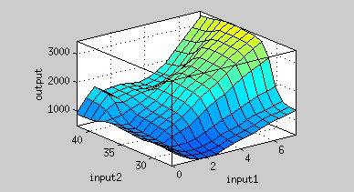
Figure 4 is the resultant graph from input 1 (time) and input 2 (AHL concentration). According to this graph, we can observe the output (fluorescence) has two peaks about AHL concentration(at concentration of 4 nM and 40 nM). That means we could achieve our regulation goal with little AHL. Also, pleas note that there is more output as time passes.
37 °C RBS
We used Figure 1 biobrick to model our 37oC RBS's function at different temperatures.
First, we did a experiment that test the fluroscence at different temperature and different time. Then we input these sets of data to ANFIS system to model the graph like Figure 2.
From Figure 1, the maximum output is obtained at 37 oC. Under the same time frame, the output (the normalized expression of the reporter gene) is maximized at 37 oC while minimized at 25 oC. There is a dramatic decrease in the output below 30 oC and the outputs around 37oC are much higher. This modeling demonstrates that using 37 oC RBS is a plausible approach for achieving gene expression through temperature.
Ecolightuner Simulation
We have all the modeling of each single unit . Now, we want to combine each unit to make a stimulation to the E.colightuner.
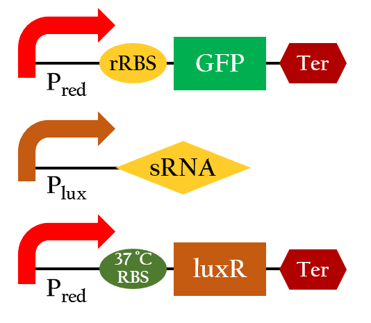
Figure 1 shows the essential constituent of our E. colightuner. To save our efforts experimenting with this essential engine of E. colightuner, we built a model beforehand to help us evaluate its practicability. Our model is consisted of three components A, B, C, and D
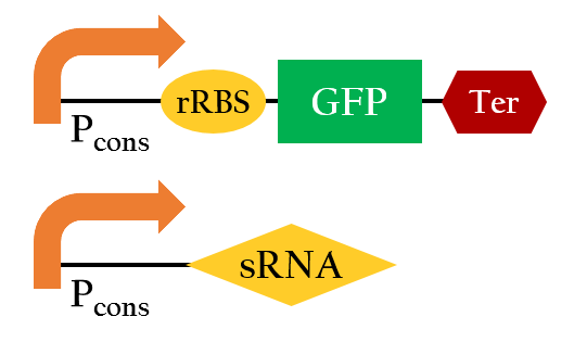
Figure 2 is the overall picture of our component A. Notice that component A is built from similar biobricks as our E.colightuner. The only difference between the two is the promoters used. Both Pred of E.colightuner are substituted with Pcons in component A. With that said, by taking the difference in the strength between Pred and Pcons, into calculations, we would be able to model out E. colightuner with component A. Before that, however, we would have to first build a model for component A.
To build a model for component A, we combined component B and C. As you can see in component B shown in Figure 3, it does not include Plux and luxR like component A. By assuming that when luxR is expressed, Plux would immediately reach its full strength, however, we can consider luxR and Plux pair as simply a Pcons,that is constitutively activated. From this perspective, component A and B are the same, except that component A is also effected by the translation efficiency of 37oC RBS. Component C in Figure 4 is the model for 37oC RBS. So by multiplying component C and component B, we would be able to obtain a model for component A.
File:NCTU A simulated-value.jpgFile:NCTU A experimental-value.jpgFile:NCTU A modified-value.jpg
In order to increase the accuracy of our component A model, we used ANFIS to fit our modeling result with the actual experimental data of our component A. By doing this, we obtained a new modeling curve for component that is more precise and accurate, shown in Figure 5.
As mentioned above, we needed to take the effect of Pred into account before we could a model of E.colightuner based on component A. Component D in Figure 6, is the model of Pred built in a similar way as component A model. We first built a model for Pred and fitted it into the actual experimental data.
Having both precise model for component A and component D, we simply had to multiple them to obtain the final model for our E.Colightuner.
 "
"


