Team:Shenzhen BGIC ATCG/Modeling
From 2013.igem.org
(→HOW TO BUILD IT) |
(→HOW TO BUILD IT) |
||
| Line 79: | Line 79: | ||
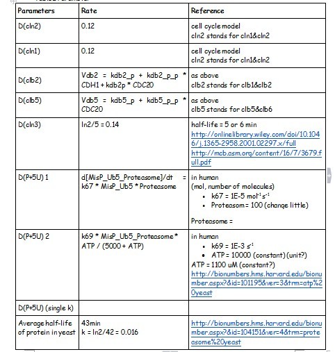
After creating the basic framework for the model we needed to create mathematical equations for each reaction with appropriate rate constants. These equations and the corresponding values are shown below in Tables 1 | After creating the basic framework for the model we needed to create mathematical equations for each reaction with appropriate rate constants. These equations and the corresponding values are shown below in Tables 1 | ||
| + | |||
| + | Table1 parameters | ||
[[File:Degradation_paramete.jpg]] | [[File:Degradation_paramete.jpg]] | ||
Revision as of 03:49, 18 September 2013
| Home | Team | Official Team Profile | Project | Parts Submitted to the Registry | Modeling | Notebook | Human Practice | Safety | Acknowledgment |
|---|
Contents |
BLUEPRINT
Our project based a lot on cell cycle, especially the cyclin-promoters and cyclin-degradation tags. Through modelling Cell cycle is one of the most complex network in biology world. Better understanding of cell cycle and it’s regulation, to some extent, faciliate the fermentation industry because we can easily accelarate or decelarate a cell cycle or even one phase in the cycle which are important for metabolism product synthesis. In order to simulation and predict the experimets of the effeciency of Sic1, alternative splicing and degradation tags in the whole cell cycle, we build tree ordinary differential equation system models.
CELL CYCLE
HOW TO BUILD IT
Using the MATLAB we created a framework of the nature cell cycle system (Figure 1). We started at the genetic level, modelling transcription, translation, phosphoralation and the degradation. We also included the rate of transport of the substrate into the cell and the diffusion of the product out of the cell. The degradation reactions for the RNA transcript and the enzyme were also included.
- SUPPOSED TO BE THE CIRCUITS******************************
After creating the basic framework for the model we needed to create mathematical equations for each reaction with appropriate rate constants. These equations and the corresponding values are shown below in Tables 1 and 2.
WHAT IT SHOWS
Before running the model we needed to decide what an appropriate endpoint would be. As we were trying to determine how quickly we could get a result we chose 2µM as our endpoint. This was chosen because initial electrochemical testing of PNP showed strong responses at concentrations as low as this. With our endpoint chosen the model was run and the data is shown below in Figure 2.
CELL CYCLE REGULATION
HOW TO BUILD IT
Using the MATLAB we created a framework of the nature cell cycle system (Figure 1). We started at the genetic level, modelling transcription, translation, phosphoralation and the degradation. We also included the rate of transport of the substrate into the cell and the diffusion of the product out of the cell. The degradation reactions for the RNA transcript and the enzyme were also included.
- SUPPOSED TO BE THE CIRCUITS******************************
After creating the basic framework for the model we needed to create mathematical equations for each reaction with appropriate rate constants. These equations and the corresponding values are shown below in Tables 1 and 2.
WHAT IT SHOWS
Before running the model we needed to decide what an appropriate endpoint would be. As we were trying to determine how quickly we could get a result we chose 2µM as our endpoint. This was chosen because initial electrochemical testing of PNP showed strong responses at concentrations as low as this. With our endpoint chosen the model was run and the data is shown below in Figure 2.
Alternative Splicing by CRISPRi
HOW TO BUILD IT
Using the MATLAB we created a framework of the nature cell cycle system (Figure 1). We started at the genetic level, modelling transcription, translation, phosphoralation and the degradation. We also included the rate of transport of the substrate into the cell and the diffusion of the product out of the cell. The degradation reactions for the RNA transcript and the enzyme were also included.
- SUPPOSED TO BE THE CIRCUITS******************************
After creating the basic framework for the model we needed to create mathematical equations for each reaction with appropriate rate constants. These equations and the corresponding values are shown below in Tables 1 and 2.
WHAT IT SHOWS
Before running the model we needed to decide what an appropriate endpoint would be. As we were trying to determine how quickly we could get a result we chose 2µM as our endpoint. This was chosen because initial electrochemical testing of PNP showed strong responses at concentrations as low as this. With our endpoint chosen the model was run and the data is shown below in Figure 2.
Degradation Rate
HOW TO BUILD IT
Using the MATLAB we created a framework of the nature cell cycle system (Figure 1). We started at the genetic level, modelling transcription, translation, phosphoralation and the degradation. We also included the rate of transport of the substrate into the cell and the diffusion of the product out of the cell. The degradation reactions for the RNA transcript and the enzyme were also included.
- SUPPOSED TO BE THE CIRCUITS******************************
After creating the basic framework for the model we needed to create mathematical equations for each reaction with appropriate rate constants. These equations and the corresponding values are shown below in Tables 1
WHAT IT SHOWS
Before running the model we needed to decide what an appropriate endpoint would be. As we were trying to determine how quickly we could get a result we chose 2µM as our endpoint. This was chosen because initial electrochemical testing of PNP showed strong responses at concentrations as low as this. With our endpoint chosen the model was run and the data is shown below in Figure 2.
 "
"
