 "
"
Team:KU Leuven/Project/Oscillator/Modelling
From 2013.igem.org


Secret garden
Congratulations! You've found our secret garden! Follow the instructions below and win a great prize at the World jamboree!
- A video shows that two of our team members are having great fun at our favourite company. Do you know the name of the second member that appears in the video?
- For one of our models we had to do very extensive computations. To prevent our own computers from overheating and to keep the temperature in our iGEM room at a normal level, we used a supercomputer. Which centre maintains this supercomputer? (Dutch abbreviation)
- We organised a symposium with a debate, some seminars and 2 iGEM project presentations. An iGEM team came all the way from the Netherlands to present their project. What is the name of their city?
Now put all of these in this URL:https://2013.igem.org/Team:KU_Leuven/(firstname)(abbreviation)(city), (loose the brackets and put everything in lowercase) and follow the very last instruction to get your special jamboree prize!


Oscillator: Model
In this part of the wiki we will describe how we performed an analysis of our proposed oscillating system and the results. This text starts with a small introduction on what we want to achieve with this oscillator, a topic that is more thoroughly elaborated on the design page. Before we started the analysis that is stated here, we looked up how similar networks have been analyzed before in order to see what direction we will take. A full-scale analysis would go beyond the scope of the project so we will stick to an elaborate indicative study. The first step is to translate our network into ODE’s (ordinary differential equations), which we will make more realistic step by step. We will use these to see how easily sustained oscillations form. This is of course not the most impressive feature since there are many known networks that easily produce oscillations. We chose not to include the effect on amplitude and frequency, since that would make the scope of this study explode and the many assumptions we have to make, render it unrealistic. The important feature of our network is its synchronization features. In order to check whether our model achieves rapid resynchronization, we will solve systems of PDE’s (partial differential equations). Since those are a lot more computationally intense, we used the Flemish Super Computer Centre (VSC) in order to do our computations time-efficiently. The explanation of how the network functions and how it attains synchronized oscillations can be found on the page explaining the design. For the transformation into a biological network, we refer you to the wetlab page.
Exploring our possibilities
Firstly, it is important to clarify what we exactly mean with ‘parameter’. A biochemical system has a very high variability in ranges for transcription rates, translation rates, degradation rates, etc. On top of that these parameters are not perfectly quantified and are subject to changes in the conditions. We checked what part of the parameter space (Box 1) creates oscillations. There are possibilities for doing this in a purely mathematical manner. Tyson (2002) gives a good example of how to study systems that produce biochemical oscillations. Polynikis, Hogan and Bernardo (2009) described modelling approaches for gene regulatory networks more generally. This is typically done by investigating the eigenvalues of the Jacobian matrix of the system. This becomes increasingly more difficult when the number of parameters and variables increases. A high level of non-linearity complicates the study of the behavior even further. In order to see what is possible we contacted Professor Dirk Roose, an expert in non-linear systems analysis. We explained him we want to investigate what parameter values create a synchronized oscillation. However, our parameter space consists of about 20 parameters that can each vary with more than a factor ten. On top of that we will have highly non-linear equations. Professor Roose told us this amount of variability would make a clean-cut mathematical examination of our model impossible . Since it is not possible to reduce our parameter space, without diverting from our goal of fully studying our system, we decided to use another strategy. We will study this enormous parameter space by generating random sets of parameters throughout this space. This offers a less theoretical, nonetheless effective means of assuring this model robustly produces oscillations.
Box1 | Parameter Space
We will explain this concept with a simple example. Let’s say we want an iGEM team (our system) to develop an oscillator. Two parameters of our system will determine whether this endeavour is successful. These parameters are the number of engineers in a team and the amount of coffee they consume per engineer. As to determine the parameter space we have to find relevant ranges for each of the parameters. We assume more than 10 engineers in the iGEM team is unlikely and a coffee consumption of more than 1.2 liter per day per engineer can also be discarded. The resulting parameter space for this two-parameter model can be easily visualised by a rectangle. This resulting parameter space can be probed and the parameter values we obtained were then used in a simulation which gave as an output whether an oscillator is produced or not. In the figure below we show the result of such a random probing of the parameter space. The blue dots represent unsuccessful endeavours and the orange dots successful ones.
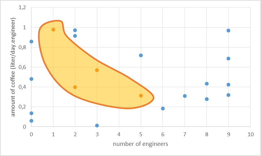 The results allow us to hypothesise on what is necessary to produce an oscillator. Apparently a higher amount of engineers still makes success possible, but only when the coffee consumption is not too high. We hypothesise here that this might be because the engineers get too much energy and start to fight amongst themselves.
We used a similar approach in the testing of our model, with some distinctions though. We deme parameter sets positive when synchronized oscillations take place. But we have 26 parameters and that makes it impossible to visualise our positive parameter space. So we chose another way to look at the parameter space and look at the total fraction of the parameter space that exhibits the wanted behaviour.
The results allow us to hypothesise on what is necessary to produce an oscillator. Apparently a higher amount of engineers still makes success possible, but only when the coffee consumption is not too high. We hypothesise here that this might be because the engineers get too much energy and start to fight amongst themselves.
We used a similar approach in the testing of our model, with some distinctions though. We deme parameter sets positive when synchronized oscillations take place. But we have 26 parameters and that makes it impossible to visualise our positive parameter space. So we chose another way to look at the parameter space and look at the total fraction of the parameter space that exhibits the wanted behaviour.
Derivation of the ordinary differential equations (ODE’s)
The preliminary system
The logical circuit of our oscillator is displayed in Figure 1 and for an elaborate explanation on this design we refer you to the design page. We will start with a preliminary translation of this network into a system of ODE’s, which is the most used method for modeling gene regulatory networks (Polynikis, Hogan and di Bernardo, 2009). An ODE cannot account for the fact that in reality each of the steps (like transcription and translation) take a finite amount of time. Danino et al. (2010) used delayed differential equations (DDE’s) as a solution for this problem but this complicates the mathematics enormously, especially when we want to take all our parameters into account. We will stick to ODE’s, since that should suffice for the study of our model. The extra delay should benefit the occurrence of oscillations because it helps diminishing peak overlap. The system of ODE’s is created by composing a rate equation for each of the six components of this preliminary circuit Figure 1. Those rate equations give the change of the components over time as a function of the amount of each of the components. The resulting system is displayed as Equation 1. Below we explain the meaning of the different components and afterwards we will explain each of the equations in this system. Further on we will derive the ODE systems for circuits that are slightly altered; by adding the fact that the production of quorum-sensing molecules goes through an enzymatic step and by using the implemented version of the OR gate.
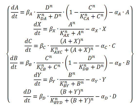 Equation 1: preliminary ODE system exhibiting the behavior of the oscillator.
The functions of the form  are called Hill functions and are often used to represent unknown regulatory functions (Rosenfeld et al., 2005). With a high Hill coefficient, represented by n in the equations above, this function approximates a step function, as can be seen in Figure 2. The other parameter of the Hill function, indicated by K, gives the moment at which half of the maximum is reached. In the ideal case of a step function, this K value gives the threshold, above which the Hill function returns 1 and below that value, the Hill function returns 0.
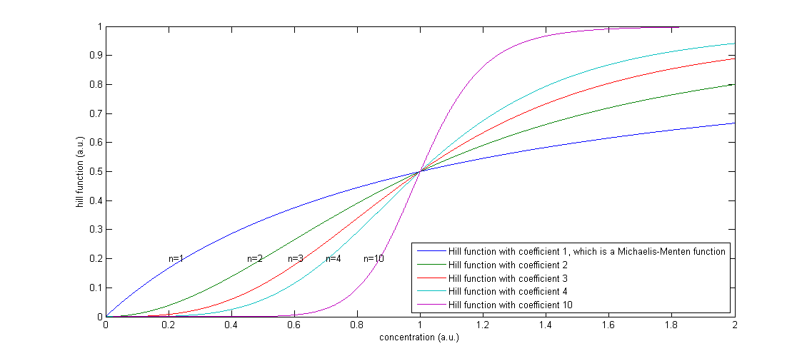 Figure 2: The effect of a higher Hill coefficient
The other parameters in this model are the maximal production rates, which are indicated by β’s and the decay rates, which are indicated by α’s. The degradation term is proportional to the concentration of that component, in which the proportionality constant α can be seen as the percentage of the present proteins that degrades in one unit of time.
We will now discuss the different rate equations and how they are linked to the logical circuit of Figure 1. The concentration of each of the components changes because of a production and a degradation term. The production depends on the presence of the other components and the degradation is as described above. Specifically for A the production is activated in the presence of D and repressed in the presence of C. The logical AND gate can be seen as if both components have to give a positive signal (presence of D and absence of C) in order to have production of A. The format 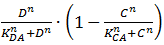 exhibits this behavior; when C is above its threshold the second term equals zero, when D is absent the first term gives zero. Consequently both D has to be present and C has to be absent to have a non-zero production term. X is a simpler case, since its production is only influenced by A; when there is a sufficient amount of A, there is production of X. C is subject to an OR gate and in order to model this we use
 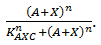 . When either A or X (or a combination of the two) reaches the required level there is production of C. For the other three rate equations the same explanation holds since it is a symmetric system.
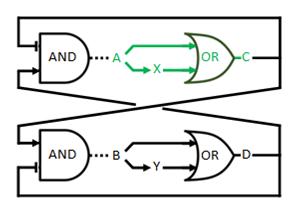
Figure 1: Logical circuit displaying our oscillator