 "
"
Team:Peking/ModelforFinetuning
From 2013.igem.org
XingjiePan (Talk | contribs) (Created page with "<html> <style type="text/css"> - →hiding the top section: body{position:absolute; top:0px; width:100%; height:1480px;} #top-section{ height:0px; border:none; width:98...") |
XingjiePan (Talk | contribs) |
||
| (69 intermediate revisions not shown) | |||
| Line 152: | Line 152: | ||
#DataPage_Sublist{position:relative; top:0px; left:-60px;} | #DataPage_Sublist{position:relative; top:0px; left:-60px;} | ||
#Safety_Sublist{position:relative; top:0px; left:-180px;} | #Safety_Sublist{position:relative; top:0px; left:-180px;} | ||
| - | #HumanPractice_Sublist{position:relative; top:0px; left:- | + | #HumanPractice_Sublist{position:relative; top:0px; left:-470px;} |
#iGEM_logo{position:absolute; top:30px; left:1090px; height:80px;} | #iGEM_logo{position:absolute; top:30px; left:1090px; height:80px;} | ||
| Line 160: | Line 160: | ||
#MajorBody{position:absolute; top:24px; left:0px; width:1200px; height:590px; background-color:#f9f9f7;} | #MajorBody{position:absolute; top:24px; left:0px; width:1200px; height:590px; background-color:#f9f9f7;} | ||
#LeftNavigation{position:fixed; top:130px; float:left; width:200px; height:100%; background-color:#313131;z-index:1000;} | #LeftNavigation{position:fixed; top:130px; float:left; width:200px; height:100%; background-color:#313131;z-index:1000;} | ||
| - | #SensorsListTitle{position:absolute; top:40px; left:20px; color:#ffffff; font-size: | + | #SensorsListTitle{position:absolute; top:40px; left:20px; color:#ffffff; font-size:20px; font-family: calibri, arial, helvetica, sans-serif; text-decoration:none; border-bottom:0px;} |
| - | #ProjectList{position:absolute; top: | + | #ProjectList{position:absolute; top:90px; left:0px; color:#ffffff; font-family: calibri, arial, helvetica, sans-serif;} |
#ProjectList > li {position:relative;display:block; list-style-type:none; width:180px; font-size:16px; text-align:left; background-color:transparent; margin:20px 0;} | #ProjectList > li {position:relative;display:block; list-style-type:none; width:180px; font-size:16px; text-align:left; background-color:transparent; margin:20px 0;} | ||
.SensorsListItem>a {color:#ffffff; text-decoration:none;} | .SensorsListItem>a {color:#ffffff; text-decoration:none;} | ||
| Line 178: | Line 178: | ||
#FixedWhiteBackground{position:fixed; top:0px; float:right; width:1200px; height:100%; z-index:-100; background-color:#ffffff;} | #FixedWhiteBackground{position:fixed; top:0px; float:right; width:1200px; height:100%; z-index:-100; background-color:#ffffff;} | ||
/*Model Editing Area*/ | /*Model Editing Area*/ | ||
| - | #ModelEditingArea{position:absolute; left:200px; top:340px; width:1000px; height: | + | #ModelEditingArea{position:absolute; left:200px; top:340px; width:1000px; height:6000px; background-color:#ffffff;font-family:calibri,Arial, Helvetica, sans-serif; font-size:18px;line-height:25px; padding:80px 0; } |
| + | .ModelEditingArea>h1{text-align:center; position:relative;left:80px; width:200px; font-size:24px;color:#FFFFFF;background-color:#004258;line-height:40px;font-weight:bold ;font-style:Italic; padding:0px;} | ||
.ModelEditingArea>p{position:relative;left:80px; width:840px; text-align:justify;} | .ModelEditingArea>p{position:relative;left:80px; width:840px; text-align:justify;} | ||
.ModelEditingArea>ol{position:relative;left:75px; width:750px; text-align:justify; font-size:16px;} | .ModelEditingArea>ol{position:relative;left:75px; width:750px; text-align:justify; font-size:16px;} | ||
.ModelEditingArea li{left:0px;} | .ModelEditingArea li{left:0px;} | ||
.ModelEditingArea a{color:#004258; font-weight:bold;} | .ModelEditingArea a{color:#004258; font-weight:bold;} | ||
| + | .ModelEditingArea table{position:relative; left:100px; width:800px; text-align:center;} | ||
| - | + | .ModelFineTFigure{position:relative; left:100px; width:800px;} | |
| - | + | ||
| - | + | ||
| - | + | ||
| - | + | ||
| - | + | ||
| - | + | ||
| - | + | ||
| - | # | + | #ModelFineTTitle1{width:200px;} |
| - | # | + | #ModelFineTTitle2{width:300px;} |
| - | + | #ModelFineTTitle3{width:430px;} | |
| - | + | #ModelFineTTitle4{width:200px;} | |
| - | + | #ModelFineTTitle5{width:300px;} | |
| - | + | #ModelFineTTitle6{width:230px;} | |
| - | + | ||
| - | + | ||
| - | + | ||
| - | + | ||
| - | # | + | |
| - | # | + | |
| - | # | + | |
| - | + | ||
| - | # | + | |
| - | + | ||
| - | + | ||
| - | + | ||
| - | + | ||
| - | + | ||
| - | + | ||
| - | + | ||
| - | + | ||
| - | + | ||
| + | #ModelFineTLegend1{position:relative; left:100px; width:800px;} | ||
| + | #ModelFineTLegend2{position:relative; left:100px; width:800px;} | ||
| + | #ModelFineTLegend3{position:relative; left:100px; width:800px;} | ||
| + | #ModelFineTLegend4{position:relative; left:100px; width:800px;} | ||
| + | #ModelFineTLegend5{position:relative; left:100px; width:800px;} | ||
| + | #ModelFineTEQ1{position:relative; left:80px; width:230px;} | ||
| + | #ModelFineTEQ2{position:relative; left:80px; width:370px;} | ||
| + | #ModelFineTEQ3{position:relative; left:80px; width:700px;} | ||
| + | #ModelFineTEQ4{position:relative; left:80px; width:500px;} | ||
| + | #ModelFineTEQ5{position:relative; left:80px; width:650px;} | ||
| + | #ModelFineTEQ6{position:relative; left:80px; width:350px;} | ||
| + | #ModelFineTEQ7{position:relative; left:80px; width:450px;} | ||
| + | #ModelFineTEQ8{position:relative; left:80px; width:450px;} | ||
| + | #ModelFineTEQ9{position:relative; left:80px; width:250px;} | ||
| + | #Figure3Complex{position:relative; height:580px;} | ||
| + | #Figure3Complex > img{position:absolute; top:0px; left:50px; width:700px;} | ||
| + | #Figure3Complex > p{position:absolute; top:320px; left:450px; width:300px;} | ||
| - | |||
| - | |||
| - | |||
| - | |||
| - | |||
| - | |||
| - | |||
| - | |||
| - | |||
| - | |||
#MileStone1{position:relative; top:-200px;} | #MileStone1{position:relative; top:-200px;} | ||
| Line 236: | Line 220: | ||
#MileStone3{position:relative; top:-200px;} | #MileStone3{position:relative; top:-200px;} | ||
#MileStone4{position:relative; top:-200px;} | #MileStone4{position:relative; top:-200px;} | ||
| + | #MileStone5{position:relative; top:-200px;} | ||
| + | #MileStone6{position:relative; top:-200px;} | ||
/*End of Model Editing Area*/ | /*End of Model Editing Area*/ | ||
| Line 261: | Line 247: | ||
</li> | </li> | ||
<li id="PKU_navbar_Team" class="Navbar_Item"> | <li id="PKU_navbar_Team" class="Navbar_Item"> | ||
| - | <a >Team</a> | + | <a href="">Team</a> |
<ul id="Team_Sublist"> | <ul id="Team_Sublist"> | ||
<div class="BackgroundofSublist"></div> | <div class="BackgroundofSublist"></div> | ||
| Line 277: | Line 263: | ||
<li><a href="https://2013.igem.org/Team:Peking/Project/Plugins">Adaptors</a></li> | <li><a href="https://2013.igem.org/Team:Peking/Project/Plugins">Adaptors</a></li> | ||
<li><a href="https://2013.igem.org/Team:Peking/Project/BandpassFilter">Band-pass Filter</a></li> | <li><a href="https://2013.igem.org/Team:Peking/Project/BandpassFilter">Band-pass Filter</a></li> | ||
| + | <li><a href="https://2013.igem.org/Team:Peking/Project/Devices">Devices</a></li> | ||
</ul> | </ul> | ||
</li> | </li> | ||
<li id="PKU_navbar_Model" class="Navbar_Item"> | <li id="PKU_navbar_Model" class="Navbar_Item"> | ||
| - | <a href=" | + | <a href="">Model</a> |
<ul id="Model_Sublist"> | <ul id="Model_Sublist"> | ||
| + | <div class="BackgroundofSublist"></div> | ||
| + | <li><a href="https://2013.igem.org/Team:Peking/Model">Band-pass Filter</a></li> | ||
| + | <li><a href="https://2013.igem.org/Team:Peking/ModelforFinetuning">Biosensor Fine-tuning</a></li> | ||
</ul> | </ul> | ||
</li> | </li> | ||
<li id="PKU_navbar_HumanPractice" class="Navbar_Item" style="width:90px"> | <li id="PKU_navbar_HumanPractice" class="Navbar_Item" style="width:90px"> | ||
| - | <a >Data page</a> | + | <a href="">Data page</a> |
<ul id="DataPage_Sublist"> | <ul id="DataPage_Sublist"> | ||
<div class="BackgroundofSublist"></div> | <div class="BackgroundofSublist"></div> | ||
| Line 302: | Line 292: | ||
<ul id="HumanPractice_Sublist"> | <ul id="HumanPractice_Sublist"> | ||
<div class="BackgroundofSublist"></div> | <div class="BackgroundofSublist"></div> | ||
| - | <li><a href="https://2013.igem.org/Team:Peking/HumanPractice/Questionnaire">Questionnaire</a></li> | + | <li><a href="https://2013.igem.org/Team:Peking/HumanPractice/Questionnaire">Questionnaire Survey</a></li> |
| - | <li><a href="https://2013.igem.org/Team:Peking/HumanPractice/FactoryVisit"> | + | <li><a href="https://2013.igem.org/Team:Peking/HumanPractice/FactoryVisit">Visit and Interview</a></li> |
<li><a href="https://2013.igem.org/Team:Peking/HumanPractice/ModeliGEM">Practical Analysis</a></li> | <li><a href="https://2013.igem.org/Team:Peking/HumanPractice/ModeliGEM">Practical Analysis</a></li> | ||
<li><a href="https://2013.igem.org/Team:Peking/HumanPractice/iGEMWorkshop">Team Communication</a></li> | <li><a href="https://2013.igem.org/Team:Peking/HumanPractice/iGEMWorkshop">Team Communication</a></li> | ||
| Line 311: | Line 301: | ||
</ul> | </ul> | ||
| - | <a href="https://igem.org/ | + | <a href="https://2013.igem.org/Main_Page"><img id="iGEM_logo" src="https://static.igem.org/mediawiki/igem.org/4/48/Peking_igemlogo.jpg"/></a> |
</div> | </div> | ||
<!--end navigationbar--> | <!--end navigationbar--> | ||
| Line 318: | Line 308: | ||
<div id="MajorBody"> | <div id="MajorBody"> | ||
<div id="LeftNavigation"> | <div id="LeftNavigation"> | ||
| - | <h1 id="SensorsListTitle"> | + | <h1 id="SensorsListTitle">Biosensor Fine-tuning</h1> |
<ul id="ProjectList"> | <ul id="ProjectList"> | ||
<li class="SensorsListItem"><a href="#MileStone1">Introduction</a><li> | <li class="SensorsListItem"><a href="#MileStone1">Introduction</a><li> | ||
| - | <li class="SensorsListItem"><a href="#MileStone2"> | + | <li class="SensorsListItem"><a href="#MileStone2">Construction of ODEs</a><li> |
| - | <li class="SensorsListItem"><a href="#MileStone3"> | + | <li class="SensorsListItem"><a href="#MileStone3">Pc Fine-tuining</a><li> |
| - | <li class="SensorsListItem"><a href="#MileStone4">Parameter | + | <li class="SensorsListItem"><a href="#MileStone4">RBS Fine-tuining</a><li> |
| + | <li class="SensorsListItem"><a href="#MileStone5">Why Medium Strength?</a><li> | ||
| + | <li class="SensorsListItem"><a href="#MileStone6">Parameter Table</a><li> | ||
</ul> | </ul> | ||
</div> | </div> | ||
<div id="ModelOverviewContainer"> | <div id="ModelOverviewContainer"> | ||
| - | <img id="ModelOverviewBackground" src="https://static.igem.org/mediawiki/ | + | <img id="ModelOverviewBackground" src="https://static.igem.org/mediawiki/2013/b/b6/Peking2013_ModelFineT_TitleBackground.png" /> |
| - | <h1 id="ModelOverviewTitle"> | + | <h1 id="ModelOverviewTitle">Biosensor Fine-tuning</h1> |
| + | |||
| Line 338: | Line 331: | ||
<!--model editing area--> | <!--model editing area--> | ||
<div id="ModelEditingArea" class="ModelEditingArea" > | <div id="ModelEditingArea" class="ModelEditingArea" > | ||
| - | + | <div id="MileStone1"></div> | |
| - | < | + | <h1 id="ModelFineTTitle1">Introduction</h1> |
| - | < | + | <p>Here we take biosensor HbpR as an example to demonstrate how our fine-tuning improves the performance of our biosensors. We constructed Ordinary Differential Equations (ODEs) based on single molecule kinetics and simulated the performance of our biosensors under different Pc and RBS strength with the steady state solution of the ODEs. </p> |
| - | + | <img class="ModelFineTFigure" src="https://static.igem.org/mediawiki/2013/8/8a/Peking2013_ModelFineT_Circuit.png" /> | |
| - | <p | + | <p id="ModelFineTLegend1"><b>Figure1.</b>Genetic regulation circuit of the biosensor HbpR.<br/><br/><br/></p> |
| - | + | ||
| - | + | <div id="MileStone2"></div> | |
| - | + | <h1 id="ModelFineTTitle2">Construction of ODEs</h1> | |
| - | + | <p>The genetic regulation circuit is shown in <b>figure 1</b> HbpR is constitutively expressed under the constitutive promoter(Pc). When the cell is exposed to its inducer X, HbpR can bind to X and form a complex HbpRX. Considering cooperation may exists in this binding reaction, the steady state concentration of HbpRX can be written as</p> | |
| - | + | <img id="ModelFineTEQ1" src="https://static.igem.org/mediawiki/2013/5/58/Peking2013_ModelFineT_EQ1.PNG" /> | |
| - | + | <p>Where K<sub>H</sub> is a constant and n<sub>H</sub> is the Hill coefficient of this reaction. | |
| - | + | <br/><br/>HbpRX is an active state, which can activate its promoter PHbpR. We assume that there are a small proportion of HbpR can change into an active state without binding to its inducer X. Therefore, the concentraion of HbpR in active state(HbpRA) can be writen as</p> | |
| - | + | <img id="ModelFineTEQ2" src="https://static.igem.org/mediawiki/2013/3/3f/Peking2013_ModelFineT_EQ2.PNG" /> | |
| - | + | <p>Where α is the proportion of HbpR in active state without binding to X. | |
| - | + | <br/><br/> | |
| - | + | HbpRA can bind to its promoter PHbpR and initiate the transcription. Concerning the number of HbpRA is much larger than the number of PHbpR the concentration of HbpRAPHbpR complex satisfies | |
| - | + | </p> | |
| - | < | + | <img id="ModelFineTEQ3" src="https://static.igem.org/mediawiki/2013/a/ae/Peking2013_ModelFineT_EQ3.PNG" /> |
| - | </ | + | <p>Where k<sub>P1</sub> and k<sub>P2</sub> are the reaction rate constants of forward and reverse reactions. |
| - | </br> | + | <br/><br/> |
| + | The concentration of mRNA satisfies | ||
| + | </p> | ||
| + | <img id="ModelFineTEQ4" src="https://static.igem.org/mediawiki/2013/c/c5/Peking2013_ModelFineT_EQ4.PNG" /> | ||
| + | <p>Where A<sub>m</sub> and D<sub>m</sub> are constants. | ||
| + | <br/><br/> | ||
| + | The concentraion of mRNA ribosome complex(mRNArib) satisfies | ||
| + | </p> | ||
| + | <img id="ModelFineTEQ5" src="https://static.igem.org/mediawiki/2013/9/91/Peking2013_ModelFineT_EQ5.PNG" /> | ||
| + | <p>Where k<sub>RBS1</sub> is the reaction rate constant of the forward reaction which is influened by the RBS strength and k<sub>R2</sub> is the reaction rate constant of the reverse reaction. | ||
| + | <br/><br/> | ||
| + | The concentration of sfGFP satisfies | ||
| + | </p> | ||
| + | <img id="ModelFineTEQ6" src="https://static.igem.org/mediawiki/2013/0/0a/Peking2013_ModerFineT_EQ6.PNG" /> | ||
| + | <p>Where A<sub>G</sub> and D<sub>G</sub> are constants. | ||
| + | <br/><br/> | ||
| + | The fluorescence can be written as | ||
</p> | </p> | ||
| - | + | <img id="ModelFineTEQ7" src="https://static.igem.org/mediawiki/2013/6/68/Peking2013_ModelFineT_EQ7.PNG" /> | |
| - | + | <p>Where A<sub>F</sub> is a constant. | |
| - | + | <br/><br/> | |
| + | We deduced the steady state solution of the ODEs above | ||
| + | </p> | ||
| + | <img id="ModelFineTEQ8" src="https://static.igem.org/mediawiki/2013/8/8e/Peking_ModelFineT_EQ8.PNG" /> | ||
| + | <p>Where</p> | ||
| + | <img id="ModelFineTEQ9" src="https://static.igem.org/mediawiki/2013/c/c3/Peking2013_ModelFineT_EQ9.PNG" /> | ||
| - | + | <p><br/><br/><br/></p> | |
| - | + | <div id="MileStone3"></div> | |
| - | + | <h1 id="ModelFineTTitle3">Constitutive Promoter Fine-tuning</h1> | |
| - | + | <p>The performance of the HbpR biosensor under different constitutive promoters are simulated by changing the parameter[HbpR](the concentration of HbpR), which variates under different strength of constitutive promoters(Pc). | |
| - | + | <br/><br/> | |
| - | + | The modeling result<b>(Figure 2)</b> shows that the fluorescence increaces as the Pc strength increaces. But a medium strength of Pc gives the highest induction ratio. | |
| - | + | ||
| - | + | ||
| - | + | ||
| - | + | ||
| - | + | ||
| - | + | ||
| - | + | ||
| - | + | ||
| - | + | ||
| - | + | ||
| - | + | ||
| - | + | ||
| - | + | ||
| - | + | ||
| - | + | ||
| - | + | ||
| - | + | ||
| - | + | ||
| - | + | ||
| - | + | ||
| - | + | ||
| - | + | ||
| - | <p | + | |
| - | + | ||
| - | + | ||
| - | + | ||
| - | + | ||
| - | + | ||
| - | + | ||
| - | + | ||
| - | + | ||
| - | + | ||
| - | + | ||
| - | + | ||
| - | + | ||
| - | + | ||
| - | + | ||
| - | + | ||
| - | + | ||
| - | + | ||
| - | + | ||
| - | + | ||
| - | + | ||
| - | + | ||
| - | + | ||
| - | + | ||
| - | + | ||
| - | + | ||
| - | + | ||
| - | + | ||
| - | + | ||
| - | + | ||
| - | + | ||
| - | + | ||
| - | + | ||
| - | + | ||
| - | + | ||
| - | + | ||
| - | + | ||
| - | + | ||
| - | + | ||
| - | + | ||
| - | + | ||
| - | + | ||
| - | + | ||
| - | + | ||
| - | + | ||
| - | + | ||
| - | + | ||
| - | + | ||
| - | + | ||
| - | + | ||
</p> | </p> | ||
| + | <img class="ModelFineTFigure" src="https://static.igem.org/mediawiki/2013/d/d7/Peking2013_ModelFineT_Figure2.png" /> | ||
| + | <p id="ModelFineTLegend2"><b>Figure 2.</b> The modeling result of the constitutive promoter fine-tuning. The dose-response curve is shown in the left plot, where the asterisks are the experimental data. The induction ratio curve is shown in the right plot.<br/><br/><br/></p> | ||
| - | < | + | <div id="MileStone4"></div> |
| - | + | <h1 id="ModelFineTTitle4">RBS Fine-tuning</h1> | |
| - | + | <p>The performance of the HbpR biosensor under different ribosome binding sites(RBSs) are simulated by changing the parameter K<sub>RBS</sub>, which is determined by the strength of RBS. | |
| - | + | <br/><br/> | |
| - | + | The modeling result<b>(Figure 3)</b> shows that the fluorescence increaces as the RBS strength increaces. But a medium strength of RBS gives the highest induction ratio. | |
| - | + | ||
| - | + | ||
| - | < | + | |
| - | + | ||
| - | + | ||
| - | + | ||
| - | + | ||
| - | <p | + | |
| - | + | ||
| - | + | ||
| - | + | ||
| - | + | ||
| - | + | ||
| - | + | ||
| - | + | ||
| - | + | ||
| - | + | ||
| - | + | ||
| - | + | ||
| - | + | ||
| - | + | ||
| - | + | ||
| - | + | ||
| - | + | ||
| - | + | ||
| - | + | ||
| - | + | ||
| - | + | ||
| - | + | ||
| - | + | ||
| - | + | ||
| - | + | ||
| - | + | ||
| - | + | ||
| - | + | ||
| - | + | ||
| - | + | ||
| - | + | ||
| - | + | ||
| - | + | ||
| - | + | ||
| - | + | ||
| - | + | ||
| - | + | ||
| - | + | ||
| - | + | ||
| - | + | ||
| - | + | ||
| - | + | ||
| - | + | ||
| - | + | ||
| - | + | ||
| - | + | ||
| - | + | ||
| - | + | ||
| - | + | ||
| - | + | ||
| - | + | ||
| - | + | ||
</p> | </p> | ||
| + | <div id="Figure3Complex" class="ModelFineTFigure"> | ||
| + | <img src="https://static.igem.org/mediawiki/2013/b/bf/Peking2013_ModelFineT_Figure3.png" /> | ||
| + | <p id="ModelFineTLegend3"><b>Figure 3.</b> The modeling result for RBS fine-tuning. <b>(a)</b>, <b>(b)</b> The dose-response curve, where the asterisks are the experimental data. <b>(c)</b> The induction ratio curve.</p> | ||
| + | </div> | ||
| - | + | <p><br/><br/><br/></p> | |
| - | + | <div id="MileStone5"></div> | |
| - | <p | + | <h1 id="ModelFineTTitle5">Why Medium Strength?</h1> |
| - | + | <p>Both experimental and modeling result shows that a medium strength of Pc and RBS gives the highest induction ratio. The reason is that a medium strength balances differet leakages. Either too strong or too weak strength will aggravate the influence of a kind of leakage. | |
| - | < | + | <br><br/> |
| - | < | + | When the strength of Pc is too weak, the induction effect is too weak compared with the leakage of promoter PHbpR. When the strength of Pc is too strong, the concentration of HbpR in active state without inducer binding is high enough to saturate the promoter PHbpR <b>(Figure 4)</b>. |
| - | + | <br><br/> | |
| - | + | When the strength of RBS is too weak, the induced fluorescence is overwhelmed by the basal fluorescence. When the strength of RBS is too strong, the translation rate will be saturated by the leakage of promoter PHbpR <b>(Figure 5)</b>. | |
| - | + | ||
</p> | </p> | ||
| + | <img class="ModelFineTFigure" src="https://static.igem.org/mediawiki/2013/3/3b/Peking2013_ModelFineT_Figure4.png" /> | ||
| + | <p id="ModelFineTLegend4"><b>Figure 4.</b> Schematic plots to show why medium strength of Pc gives the highest induction ratio. In the left plot, the dose-response curve of HbpR in active state (HbpRA) under different Pc are plotted in different colors and the lower and upper bounds are denoted in a and b. The right plot shows mRNA expression level in different lower and upper bounds. The induction ratio can be calculated by dividing the fluorescence at b point by the fluorescence at a point.</p> | ||
| + | <img class="ModelFineTFigure" src="https://static.igem.org/mediawiki/2013/7/72/Peking2013_ModelFineT_Figure5.png" /> | ||
| + | <p id="ModelFineTLegend5"><b>Figure 5.</b> Schematic plots to show why medium strength of RBS gives the highest induction ratio. In the left plot, the lower and upper bound of mRNA expression level are denoted in a and b. The right plot shows the dose-response curves of mRNA under different RBSs. The induction ratio can be calculated by dividing the fluorescence at b point by the fluorescence at a point.<br/><br/><br/> </p> | ||
| + | <div id="MileStone6"></div> | ||
| + | <h1 id="ModelFineTTitle6">Parameter Table</h1> | ||
| + | <table border="1"> | ||
| + | <tr><th>Parameter</th><th>Value</th></tr> | ||
| + | <tr><td rowspan="3">[HbpR]</td><td>10000 for J23106</td></tr> | ||
| + | <tr><td>256 for J23114</td></tr> | ||
| + | <tr><td>22 for J23113</td></tr> | ||
| + | <tr><td>n<sub>H</sub></td><td>1.7</td></tr> | ||
| + | <tr><td>α</td><td>0.003</td></tr> | ||
| + | <tr><td>K<sub>H</sub></td><td>0.004</td></tr> | ||
| + | <tr><td>K<sub>PH</sub></td><td>0.005</td></tr> | ||
| + | <tr><td>K<sub>m</sub></td><td>0.005</td></tr> | ||
| + | <tr><td>Leakage</td><td>0.008</td></tr> | ||
| + | <tr><td rowspan="2">K<sub>F</sub></td><td>1400 for Pc simulation</td></tr> | ||
| + | <tr><td>1900 for RBS simulation</td></tr> | ||
| + | <tr><td rowspan="4">K<sub>RBS</sub></td><td>0.3 for Pc simulation</td></tr> | ||
| + | <tr><td>0.17 for B0034</td></tr> | ||
| + | <tr><td>3.5 for B0032</td></tr> | ||
| + | <tr><td>7 for B0031</td></tr> | ||
| + | <tr><td rowspan="2">BasalFluorescence</td><td>60 for Pc simulation</td></tr> | ||
| + | <tr><td>2 for RBS simulation</td></tr> | ||
| + | </table> | ||
| + | <p>*Parameters are determined from curve fitting. Because the experimental data of Pc fine-tuning and data of RBS fine-tuning are measured in different experiments, K<sub>F</sub> and BasalFluorescence has different value in Pc and RBS simulation.</p> | ||
| - | + | </div> | |
| - | + | ||
| - | + | ||
| - | + | ||
<!--end of model editing area--> | <!--end of model editing area--> | ||
| Line 548: | Line 460: | ||
| - | |||
| - | |||
| - | |||
| - | |||
| - | |||
| - | |||
| - | |||
| - | |||
| - | |||
| - | |||
| - | |||
| - | |||
| - | |||
| - | |||
| - | |||
| - | |||
| - | |||
| - | |||
| - | |||
| - | |||
| - | |||
| - | |||
| - | |||
| - | |||
| - | |||
| - | |||
| - | |||
| - | |||
| - | |||
| - | |||
| - | |||
| - | |||
| - | |||
| - | |||
| - | |||
| - | |||
| - | |||
| - | |||
| - | |||
| - | |||
| - | |||
| - | |||
| - | |||
| - | |||
| - | |||
| - | |||
| - | |||
| - | |||
| - | |||
| - | |||
| - | |||
| - | |||
| - | |||
| - | |||
| - | |||
| - | |||
| - | |||
| - | |||
| - | |||
| - | |||
| - | |||
| - | |||
| - | |||
| - | |||
| - | |||
| - | |||
| - | |||
| - | |||
| - | |||
| - | |||
| - | |||
| - | |||
| - | |||
| - | |||
| - | |||
| - | |||
| - | |||
| - | |||
| - | |||
| - | |||
| - | |||
| - | |||
| - | |||
| - | |||
| - | |||
| - | |||
| - | |||
| - | |||
| - | |||
| - | |||
| - | |||
| - | |||
| - | |||
| - | |||
| - | |||
| - | |||
| - | |||
| - | |||
| - | |||
| - | |||
| - | |||
| - | |||
| - | |||
| - | |||
| - | |||
| - | |||
| - | |||
| - | |||
| - | |||
| - | |||
| - | |||
| - | |||
| - | |||
| - | |||
| - | |||
| - | |||
| - | |||
| - | |||
| - | |||
| - | |||
| - | |||
| - | |||
| - | |||
| - | |||
| - | |||
| - | |||
| - | |||
| - | |||
| - | |||
| - | |||
| - | |||
| - | |||
| - | |||
| - | |||
| - | |||
| - | |||
| - | |||
| - | |||
| - | |||
| - | |||
| - | |||
| - | |||
| - | |||
| - | |||
| - | |||
| - | |||
| - | |||
| - | |||
| - | |||
| - | |||
| - | |||
| - | |||
| - | |||
| - | |||
| - | |||
| - | |||
| - | |||
| - | |||
| - | |||
| - | |||
| - | |||
Latest revision as of 18:17, 28 October 2013


Biosensor Fine-tuning
Introduction
Here we take biosensor HbpR as an example to demonstrate how our fine-tuning improves the performance of our biosensors. We constructed Ordinary Differential Equations (ODEs) based on single molecule kinetics and simulated the performance of our biosensors under different Pc and RBS strength with the steady state solution of the ODEs.
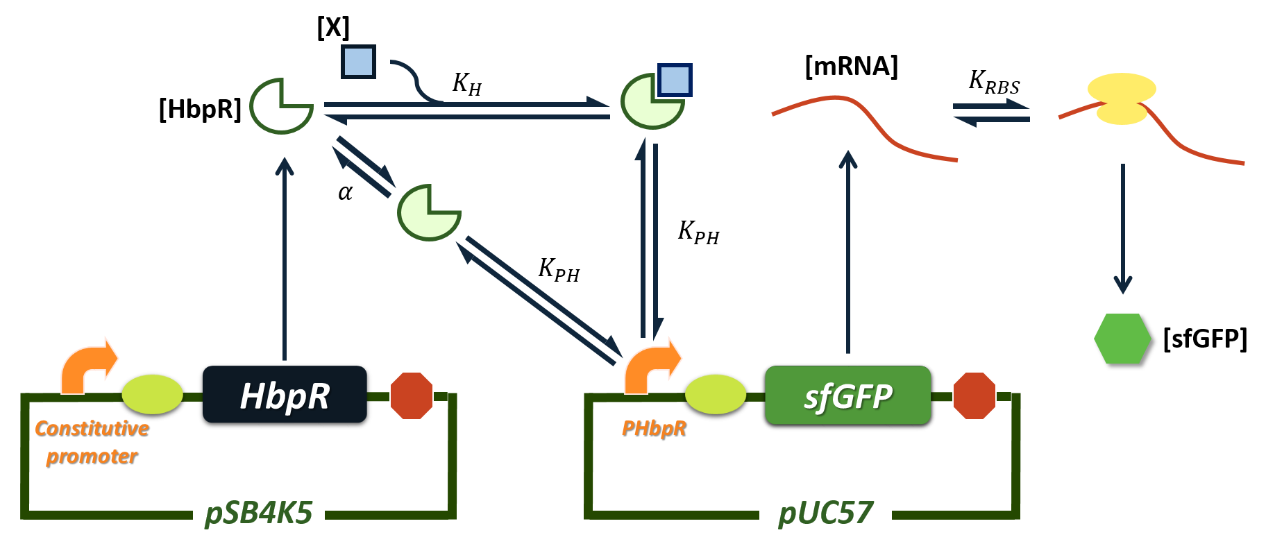
Figure1.Genetic regulation circuit of the biosensor HbpR.
Construction of ODEs
The genetic regulation circuit is shown in figure 1 HbpR is constitutively expressed under the constitutive promoter(Pc). When the cell is exposed to its inducer X, HbpR can bind to X and form a complex HbpRX. Considering cooperation may exists in this binding reaction, the steady state concentration of HbpRX can be written as
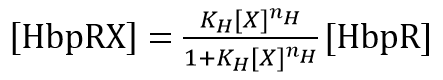
Where KH is a constant and nH is the Hill coefficient of this reaction.
HbpRX is an active state, which can activate its promoter PHbpR. We assume that there are a small proportion of HbpR can change into an active state without binding to its inducer X. Therefore, the concentraion of HbpR in active state(HbpRA) can be writen as
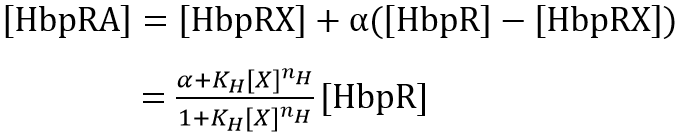
Where α is the proportion of HbpR in active state without binding to X.
HbpRA can bind to its promoter PHbpR and initiate the transcription. Concerning the number of HbpRA is much larger than the number of PHbpR the concentration of HbpRAPHbpR complex satisfies

Where kP1 and kP2 are the reaction rate constants of forward and reverse reactions.
The concentration of mRNA satisfies

Where Am and Dm are constants.
The concentraion of mRNA ribosome complex(mRNArib) satisfies

Where kRBS1 is the reaction rate constant of the forward reaction which is influened by the RBS strength and kR2 is the reaction rate constant of the reverse reaction.
The concentration of sfGFP satisfies
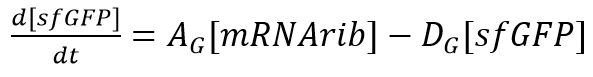
Where AG and DG are constants.
The fluorescence can be written as

Where AF is a constant.
We deduced the steady state solution of the ODEs above
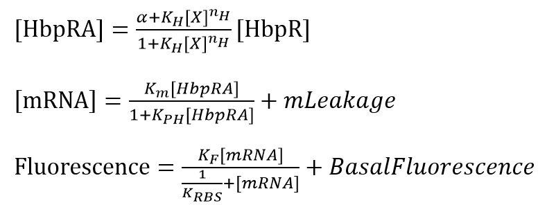
Where
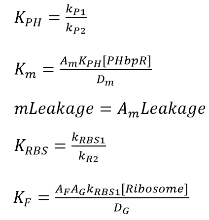
Constitutive Promoter Fine-tuning
The performance of the HbpR biosensor under different constitutive promoters are simulated by changing the parameter[HbpR](the concentration of HbpR), which variates under different strength of constitutive promoters(Pc).
The modeling result(Figure 2) shows that the fluorescence increaces as the Pc strength increaces. But a medium strength of Pc gives the highest induction ratio.
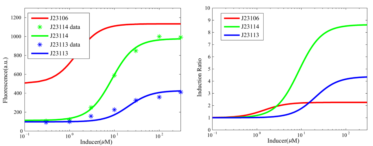
Figure 2. The modeling result of the constitutive promoter fine-tuning. The dose-response curve is shown in the left plot, where the asterisks are the experimental data. The induction ratio curve is shown in the right plot.
RBS Fine-tuning
The performance of the HbpR biosensor under different ribosome binding sites(RBSs) are simulated by changing the parameter KRBS, which is determined by the strength of RBS.
The modeling result(Figure 3) shows that the fluorescence increaces as the RBS strength increaces. But a medium strength of RBS gives the highest induction ratio.
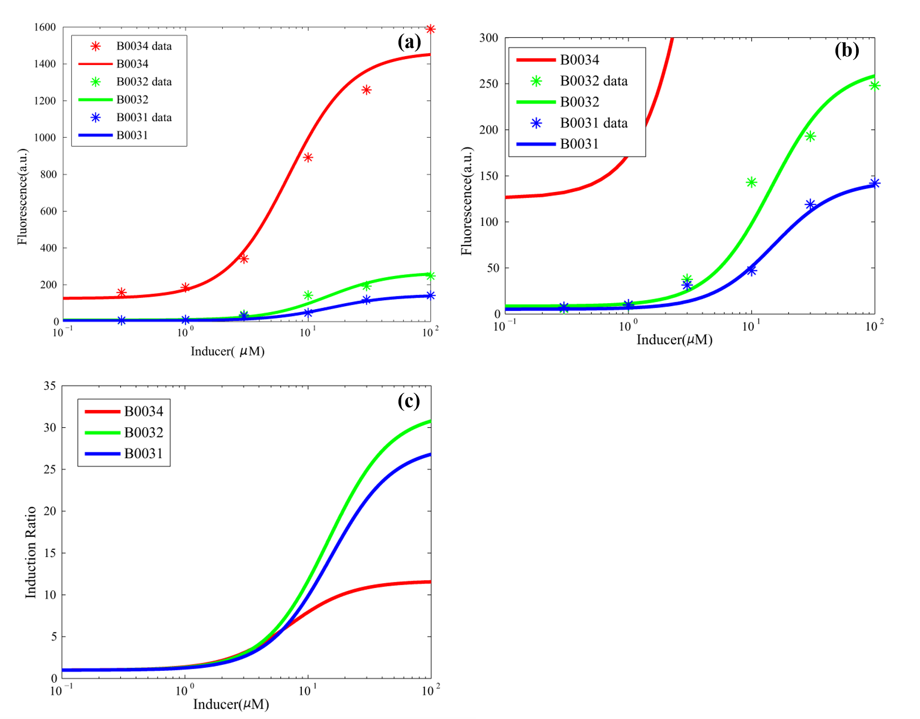
Figure 3. The modeling result for RBS fine-tuning. (a), (b) The dose-response curve, where the asterisks are the experimental data. (c) The induction ratio curve.
Why Medium Strength?
Both experimental and modeling result shows that a medium strength of Pc and RBS gives the highest induction ratio. The reason is that a medium strength balances differet leakages. Either too strong or too weak strength will aggravate the influence of a kind of leakage.
When the strength of Pc is too weak, the induction effect is too weak compared with the leakage of promoter PHbpR. When the strength of Pc is too strong, the concentration of HbpR in active state without inducer binding is high enough to saturate the promoter PHbpR (Figure 4).
When the strength of RBS is too weak, the induced fluorescence is overwhelmed by the basal fluorescence. When the strength of RBS is too strong, the translation rate will be saturated by the leakage of promoter PHbpR (Figure 5).
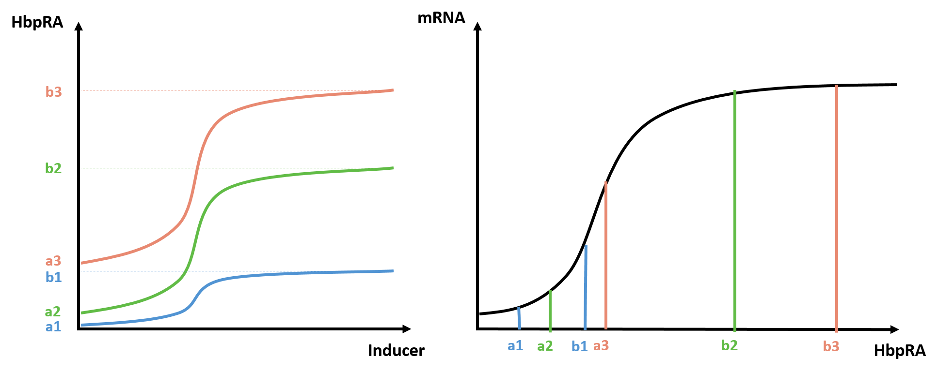
Figure 4. Schematic plots to show why medium strength of Pc gives the highest induction ratio. In the left plot, the dose-response curve of HbpR in active state (HbpRA) under different Pc are plotted in different colors and the lower and upper bounds are denoted in a and b. The right plot shows mRNA expression level in different lower and upper bounds. The induction ratio can be calculated by dividing the fluorescence at b point by the fluorescence at a point.

Figure 5. Schematic plots to show why medium strength of RBS gives the highest induction ratio. In the left plot, the lower and upper bound of mRNA expression level are denoted in a and b. The right plot shows the dose-response curves of mRNA under different RBSs. The induction ratio can be calculated by dividing the fluorescence at b point by the fluorescence at a point.
Parameter Table
| Parameter | Value |
|---|---|
| [HbpR] | 10000 for J23106 |
| 256 for J23114 | |
| 22 for J23113 | |
| nH | 1.7 |
| α | 0.003 |
| KH | 0.004 |
| KPH | 0.005 |
| Km | 0.005 |
| Leakage | 0.008 |
| KF | 1400 for Pc simulation |
| 1900 for RBS simulation | |
| KRBS | 0.3 for Pc simulation |
| 0.17 for B0034 | |
| 3.5 for B0032 | |
| 7 for B0031 | |
| BasalFluorescence | 60 for Pc simulation |
| 2 for RBS simulation |
*Parameters are determined from curve fitting. Because the experimental data of Pc fine-tuning and data of RBS fine-tuning are measured in different experiments, KF and BasalFluorescence has different value in Pc and RBS simulation.
