Selecting Network Topologies

There are a lot of potential band-pass filter circuit networks with an incoherent feed-forward loop (for specific definition, view Project, band-pass filter ) as its core topology. The simplest one is a two-node network consisting of a positive loop and a negative loop (Fig 1.a). But it’s too difficult to make a transcriptional factor both activator and repressor at the same time. So we discarded such a network despite it simplicity.

So we set out to look for topologies with three or more nodes based on two criteria: first, considering functioning mechanisms of real protein regulators, the input node must regulate other nodes in a uniform manner, either all inhibiting or all promoting; second, to lessen the manual work required to construct the circuit, we require both the positive and negative feed-forward loop to contain no more than one internode. In the end, we decided to analyze three topologies in detail, two of them have three nodes and one has four nodes (Fig 1.b, c, d).

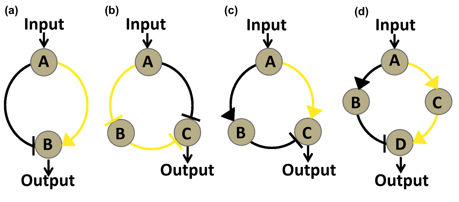
Figure 1. Four circuit networks we considered in our modeling. Each node represent a regulatory protein, either an activator or and repressor. All four networks possess incoherent feed-forward loops as core topology. Components of the activating half of an incoherent feed-forward loop are marked as green while components of repressing half are marked as black. a. The simplest two node circuit possessing an incoherent feed-forward loop. In this network, Input node A functions both as an activator and an repressor, so it has to be eliminated. b, c, Three-node networks taken into consideration. The principal difference between these two networks is the regulatory function of input node A. b, Three-node network where input node A functions as repressor. A directly repress output node C while indirectly activating it by inhibiting B, which represses C directly. c, Three-node network where input node A functions as activator. A directly repress output node C while indirectly activating it by activating B, which represses C directly. d, Four-node network taken into consideration. A indirectly activates output node D by activating C which activates D, while indirectly represses output by activating B that inhibits D.

ODE Analysis of Circuit Networks

After determining three typical circuit networks that might function as band-pass filters, we used Ordinary Differential Equations (ODE) to analyze the three topology and their parameter preferences.

Our ODE model of the circuit networks was established based on the following assumptions:

1. Only transcription and translation process is taken into consideration. The equations only contain accumulation and degradation of the proteins represented by the nodes.
2. The interactions between nodes are described using Hill functions. We multiplied the Hill functions describing the individual regulating effects of activator and repressor in order to simulate the synergic regulating effect of the two transcription factors when bound to the same promoter.
3. The protein represented by the input node is constitutively expressed at a fixed level.
4. Leakage is present only in the expression of reporter gene (output node).

The ODE equations we used to simulate the three circuit networks are listed as following:

Circuit Network 1:

Note: Since A is expressed at a fixed level, its influence on the network can be absorbed into other constants in the model, so it doesn't appear in the equations written above.

Letting the differential term on the left handed side equal to zero, the steady state solution of the equations can be solved as following:

Circuit Network 2:

Note: For reason same as that described in Circuit Network 1, expression level of A doesn't appear in the equations written above.

The steady state solution of the equations can be solved as following:

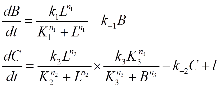
Circuit Network 3:

Note: For reason same as that described in Circuit Network 1, expression level of A doesn't appear in the equations written above.

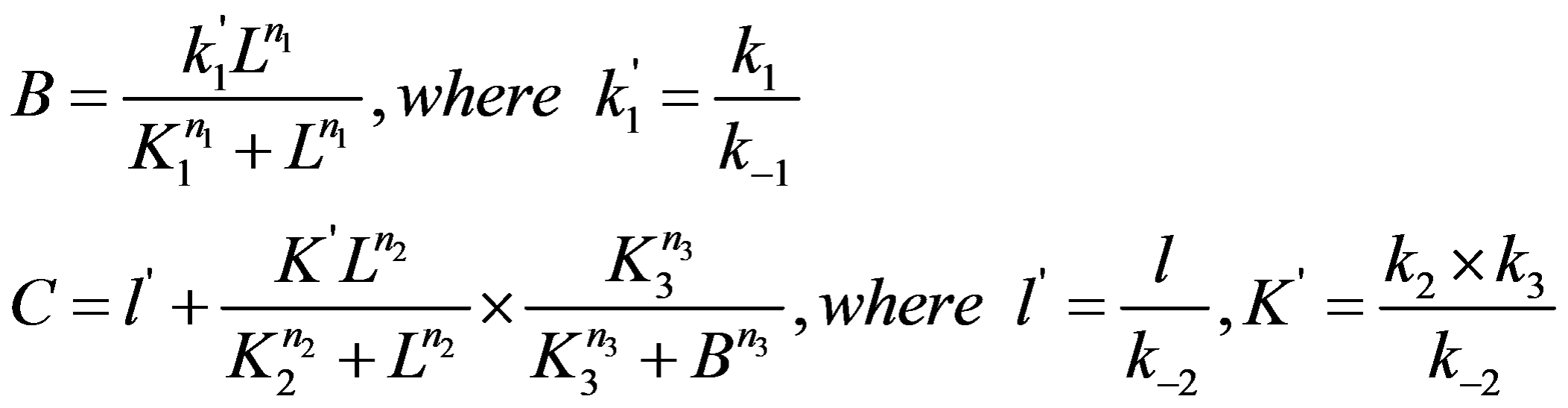
The steady state solution of the equations can be solved as following:

In the equations written above, k in lowercase are used to denote maximum expression rate constant of individual regulation loops. k in uppercase are used to denote the transition point of different Hill functions. A, B, C, D are used to denote expression level of proteins represented by corresponding nodes. n in lowercase denote Hill coefficient of different Hill functions. l in lowercase denote leakage terms.
The next step is to use ODE equations given above to find out the most robust circuit network. In order to do this, we applied 10,000 sets of randomly sampled network parameters to each of the three topologies and evaluated their behavior according to two important features: induction fold and peak width (Fig. ). Parameter sets resulting in a high induction fold (>32) and a reasonable peak width (<4&>0.5) are recorded separately for each topology.

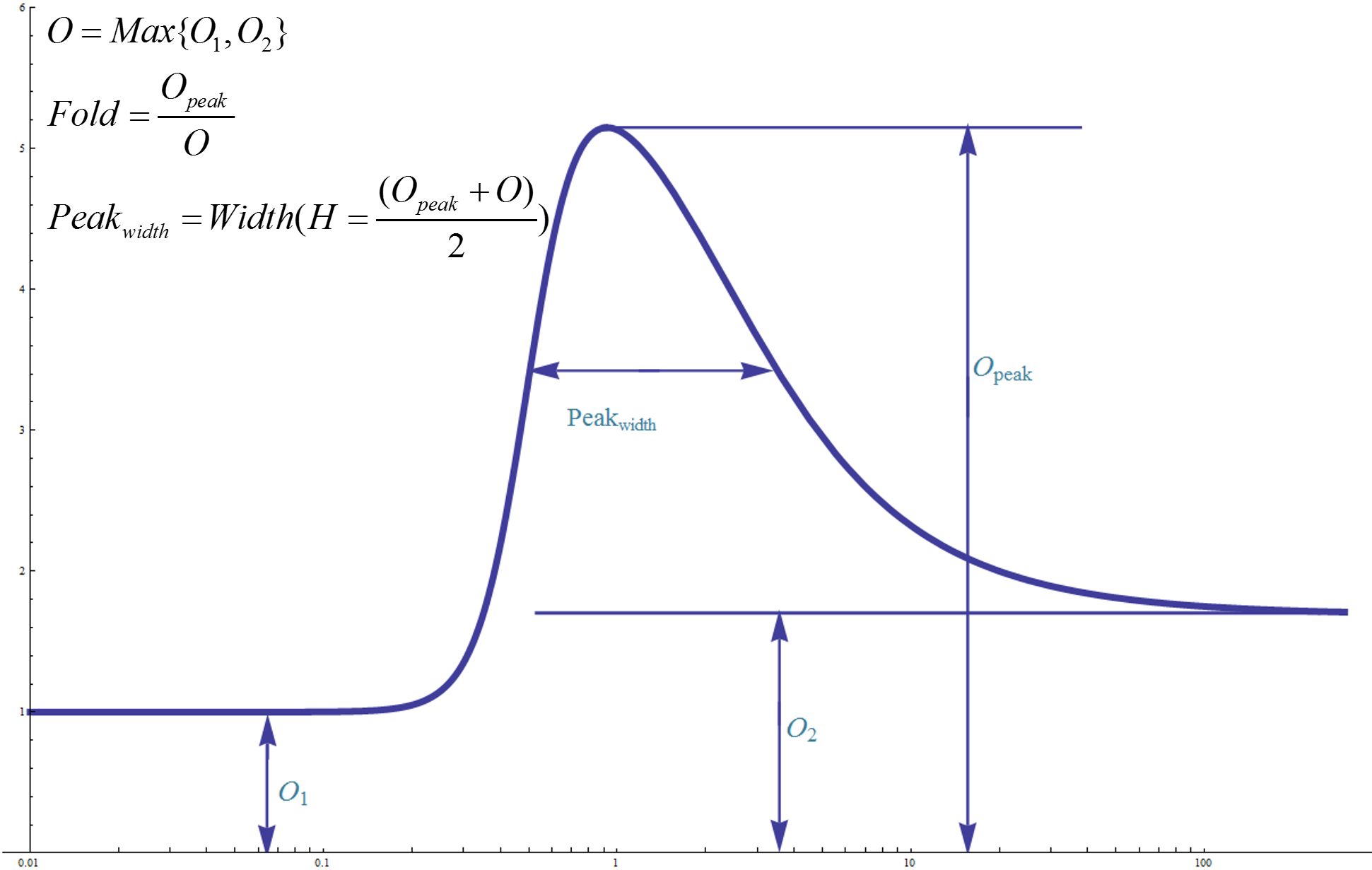
Figure 2. Graph illustration of the definition of induction fold and peak width. Left basal value O₁ equals to y-axis intercept of the dose-response curve's horizontal asymptotic line as input intensity tends to zero. Right basal value O₂ equals to y-axis intercept of the dose-response curve's horizontal asymptotic line as input intensity tends to infinity. Effective basal value O is defined as the greater one among O₁ and O₂. O_peak equals to peak value of the dose-response curve. Induction ration equals to O_peak divided by O. Peak width is defined as the distance between the two points with y coordinate equal to (O_peak+O)/2. Induction fold and peak width is the two most important judging criteria used in our modeling.

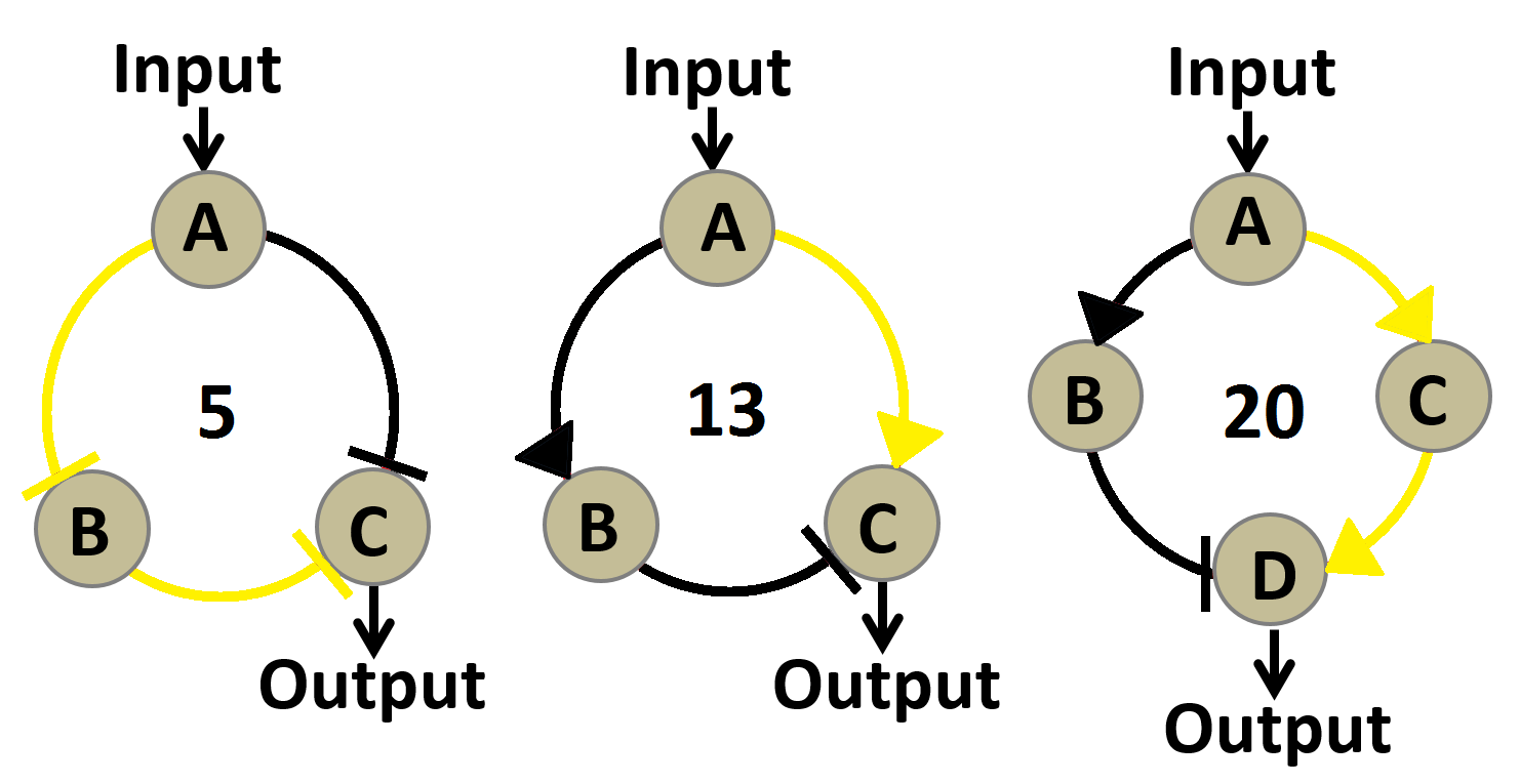
Figure 3.Three circuit networks we evaluated in our ODE based robustness analysis. The number of parameter sets capable of generating desirable induction fold and peak width (fold>32 and 4>peak width>0.5) are written in the middle of each network graph. A larger number of effective parameter sets indicates a more robust circuit network.

Results of robustness analysis are shown in Figure 2. 20 out 10000 sets of parameters applied to circuit network 3 generated a desirable performance. The number of effective parameter sets for circuit network 1 and 2 are 5 and 13 respectively. This indicates that circuit network 3 may function in a larger proportion of the parameter space, meaning it would be more likely than the other two to work well in noisy biological context and might require less effort on fine-tuning individual components of the circuit network. So we chose the third circuit network as the blueprint for our band-pass filter.

Parameter Sensitivity Analysis

Having decided which circuit network to use, our next move is to determine which proteins to choose for individual nodes in the circuit network to construct a band-pass filter. First we decided to use parameter sensitivity analysis to figure out which parameters in the circuit network are most sensitive to perturbation. These parameters are crucial for own design because they must be carefully controlled within a narrow range to make sure our circuit would function properly. Once we have figured out all sensitive parameters, we may facilitate our design by choosing proteins with desirable sensitive parameter value.

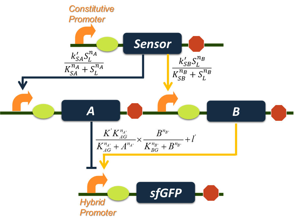
Figure 4. Blueprint for the construction of band-pass filter circuit and a graph summary of equations we use for stimulation. The sensor for input node is supposed to be a transcription regulator capable of responding to aromatic compounds, and we fixed sfGFP reporter as the output node; protein candidates for repressor node A and activator node B remain to be determined based on information gathered from parameter sensitivity analysis.

In order to be more specific in our parameter sensitivity analysis, we re-wrote the ODEs for the band-pass filter as following:

And steady state solution can be solved as following:

Symbol usages are identical to that in ODE analysis of network topologies.

We chose one set of parameters meeting our needs (peak fold>32 and 4>peak width>0.5) as our initial parameter set. We then enlarged each parameter ten times and observed the difference between pre-change behavior and post-change behavior of the band-pass filter circuit. We used log(f’/f) and log(p/p’) to characterize the change in band-pass performance, where f and f’ denote the fold change before and after parameter perturbation, p and p’ denote the peak width before and after parameter perturbation. A log(f'/f) greater than zero indicates that the induction fold has increased after the parameter perturbation, meaning the perturbation is conducive to band-pass filter's performance. A log(p/p') greater than zero indicates that the peak width has reduced after the parameter perturbation, also meaning the perturbation is desirable.

The quantitative results of parameter sensitivity analysis are shown in Figure 4 and the qualitative results are summarized in Table 1. To further help understanding we drew a series of pictures to show the how the network behaves as some of the parameters change (Fig.5).

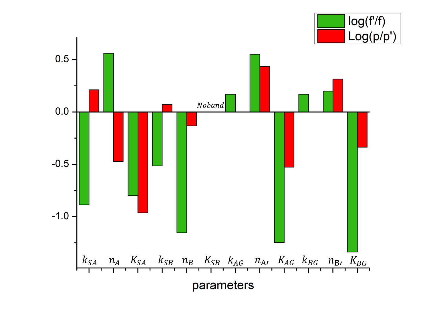
Figure 5. Fold’ (f’) and p’ indicate Fold and peak width after we changed the parameters and Fold (f) and p indicate Fold and peak width before we changed the parameters. An upward-pointing column indicates changes that are conducive to our design, and a downward-pointed column indicates changes detrimental to our design. This figure shows how the band changes with the variation of each parameter.

As can be concluded from figure 4 and table 1, parameters are sensitive to enlargement in four different ways. Some parameters, such as ksa, nb, na', Kag nb' and Kbg, once enlarged, will enhance or deteriorate the performance of induction ration and band width at the same time; another group of parameters, such as ksa, na and ksb, once enlarged, will enhance one important feature while deteriorating the other; a third group of parameters, such as kag and kbg, have little effect on one of the two important features; a final group of parameter, consisting of Ksb only, will totally eliminate the band when enlarged.

In order to tune our band pass filter most efficiently, we decided to focus on the first group of parameters because by increasing or decreasing the value of such parameters will improve the induction ratio and peak width at the same time. And since in real applications we need to change the sensor (input node) from one aromatics-responsive transcription factor to another, we don't want to set too tight a restriction on sensor-related parameters such as ksa and nb. So we limited the tunable parameters to na', nb' Kag and Kbg. As can be easily observed from figure 4, for a outstanding band-pass filter circuit, higher values for na' and nb' as well as lower values for Kag and Kbg are desirable.

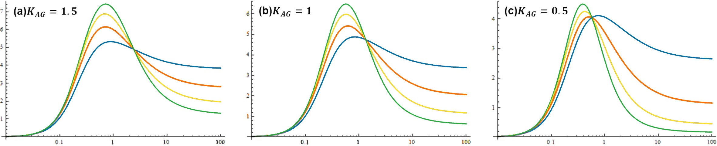
Figure 6.The dose-response curve of different sets of parameters. na’ is the hill coefficient of repressor A. KAG is the ligand concentration producing half occupation. The green line means na’=2, the yellow one means na’=1.5, the red one means na’=1 and the blue one means na’=0.5. (a)KAG=1.5(b) KAG=1(c) KAG=1.From the pictures above, we can see that a small KAG and a large na’ is needed to build a good performance band-pass filter.

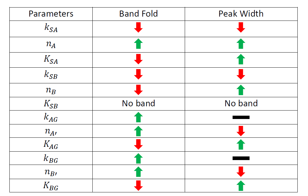
Table 1. The change of two important characters as the parameters rise. Green arrow has the meaning that the character value rises as the parameter rises. Red arrow has the reverse meaning. Black line means that the charater value keep relative stability as the parameter changes.

Based on all the analysis we have done above, we chose the activator from phage phiR73 as node B for its small dissociation constant (Kbg) and repressor form phage λ as node A for its large hill coefficient (na') to construct our final band-pass filter circuit (Fig. 5).

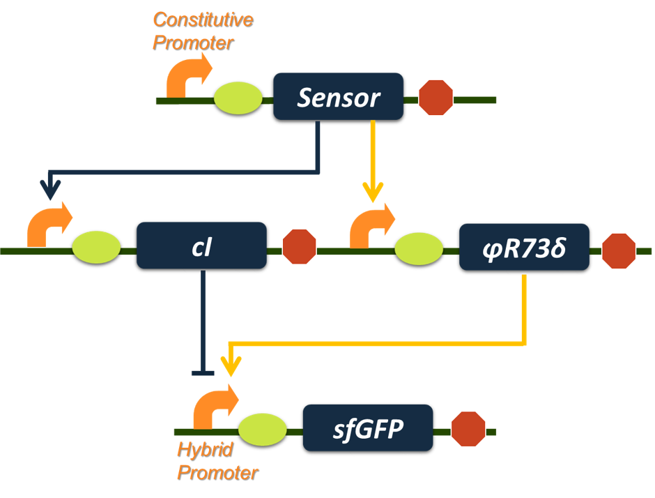
Figure 7.The final construct of our band-pass filter.