Team:Duke/Modeling/3
From 2013.igem.org
Hyunsoo kim (Talk | contribs) (→Following Gardner's Work...) |
Hyunsoo kim (Talk | contribs) (→Following Gardner's Work...) |
||
| Line 20: | Line 20: | ||
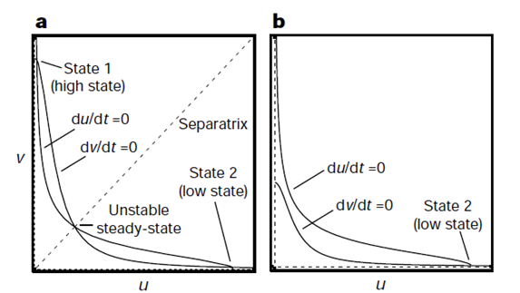
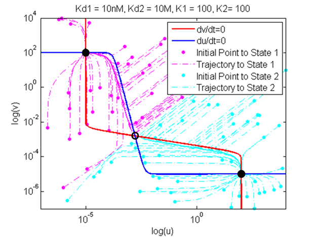
Using this model, Gardner produced the two graphs shown below. The first is a graph of nullclines. Nullcline, also called zero-growth isocline, is a line that represents the set of points at which the rate of change is zero. In this example, the two nullclines shown are where rate of change of repressor 1 (U) and repressor 2 (V) are zero. It is clear that at the intersection of these two nullclines are steady-state points of the system because these are points where the change of both repressor levels with respect to time is zero. <br><br> | Using this model, Gardner produced the two graphs shown below. The first is a graph of nullclines. Nullcline, also called zero-growth isocline, is a line that represents the set of points at which the rate of change is zero. In this example, the two nullclines shown are where rate of change of repressor 1 (U) and repressor 2 (V) are zero. It is clear that at the intersection of these two nullclines are steady-state points of the system because these are points where the change of both repressor levels with respect to time is zero. <br><br> | ||
| - | The difference between the two figures with nullclines on left and right is that the system on the left is bistable with the system on the right is mono-stable. | + | The difference between the two figures with nullclines on left and right is that the system on the left is bistable with the system on the right is mono-stable. Figure (a) shows that there are two stable steady-states where only one of the two repressors exists at a high level, inhibiting the production of the other repressor. There exists a third intersection in the middle, however, this point can be mathematically shown to be unstable using the eigenvalue of the Jacobian matrix involving U and V (workings not included here). The value of U and V doesnt change exactly at this unstable steady-state, however, the level of repressors will quickly diverge from this point even at the smallest perturbation. The figure on the right, figure (b), shows that at a different combination of parameters, a system can be mono-stable where the nullclines only intersect once at a stable steady-state solution. |
explain nullclines | explain nullclines | ||
Revision as of 05:55, 22 September 2013
Contents |
Mathematical Modeling of Bistable Toggle Switch
Kinetic Model of Bistable System
Following Gardner's Work...
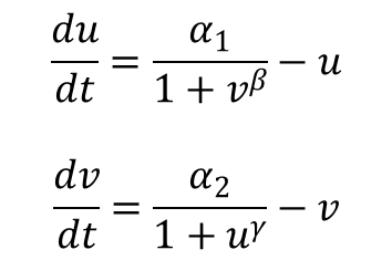
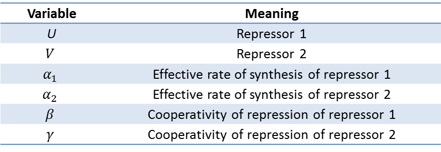
Tim Gardner from Jim Collins' Lab of Boston Univeristy published one of the first major papers on genetic toggle switch. In his work, he used a kinetic approach to model the stability of a genetic toggle switch. His equations involved two equations expressing the change in the level of two mutually repressive repressors with respect to time.
Using this model, Gardner produced the two graphs shown below. The first is a graph of nullclines. Nullcline, also called zero-growth isocline, is a line that represents the set of points at which the rate of change is zero. In this example, the two nullclines shown are where rate of change of repressor 1 (U) and repressor 2 (V) are zero. It is clear that at the intersection of these two nullclines are steady-state points of the system because these are points where the change of both repressor levels with respect to time is zero.
The difference between the two figures with nullclines on left and right is that the system on the left is bistable with the system on the right is mono-stable. Figure (a) shows that there are two stable steady-states where only one of the two repressors exists at a high level, inhibiting the production of the other repressor. There exists a third intersection in the middle, however, this point can be mathematically shown to be unstable using the eigenvalue of the Jacobian matrix involving U and V (workings not included here). The value of U and V doesnt change exactly at this unstable steady-state, however, the level of repressors will quickly diverge from this point even at the smallest perturbation. The figure on the right, figure (b), shows that at a different combination of parameters, a system can be mono-stable where the nullclines only intersect once at a stable steady-state solution.
explain nullclines explain bifurcation
figure (trajectory)
figure (bifurcation)
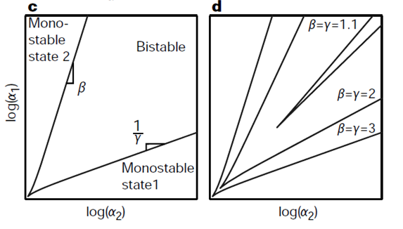
explain the effect of changing hill coeff on bifurcation region. explain nullcline
reproduce nullcline and trajectory (explain trajectory)
Development of Our Kinetic Model
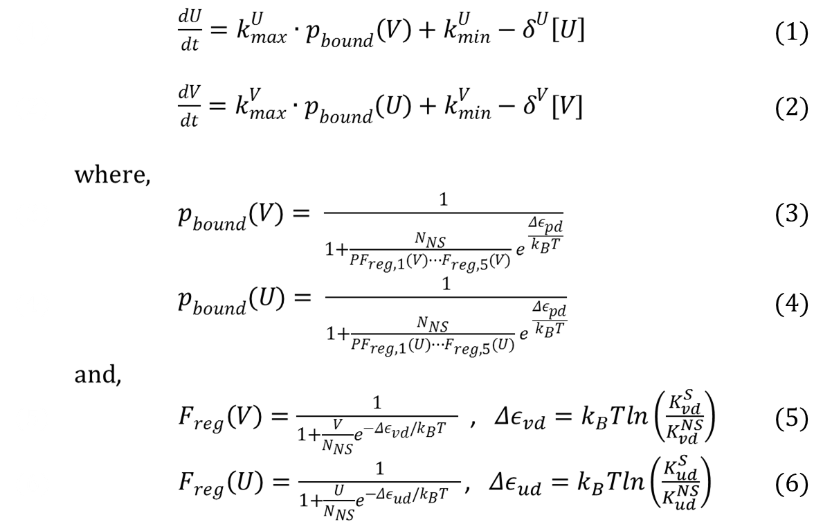
moving on, we have developed another kinetic model using the results of the thermodynamic model. gardner = effect of hill coeff on bistability of a system (bifurcation region) new model = effect of various parameters on bistability (highlight and number Kd, pr_Str, basal rate.
as mentioned before, key assumption is is (du/dt , dv/dt = proportional to p_bound)
show equation
explain
show values for variables like degradation rate
Results from Our Kinetic Model
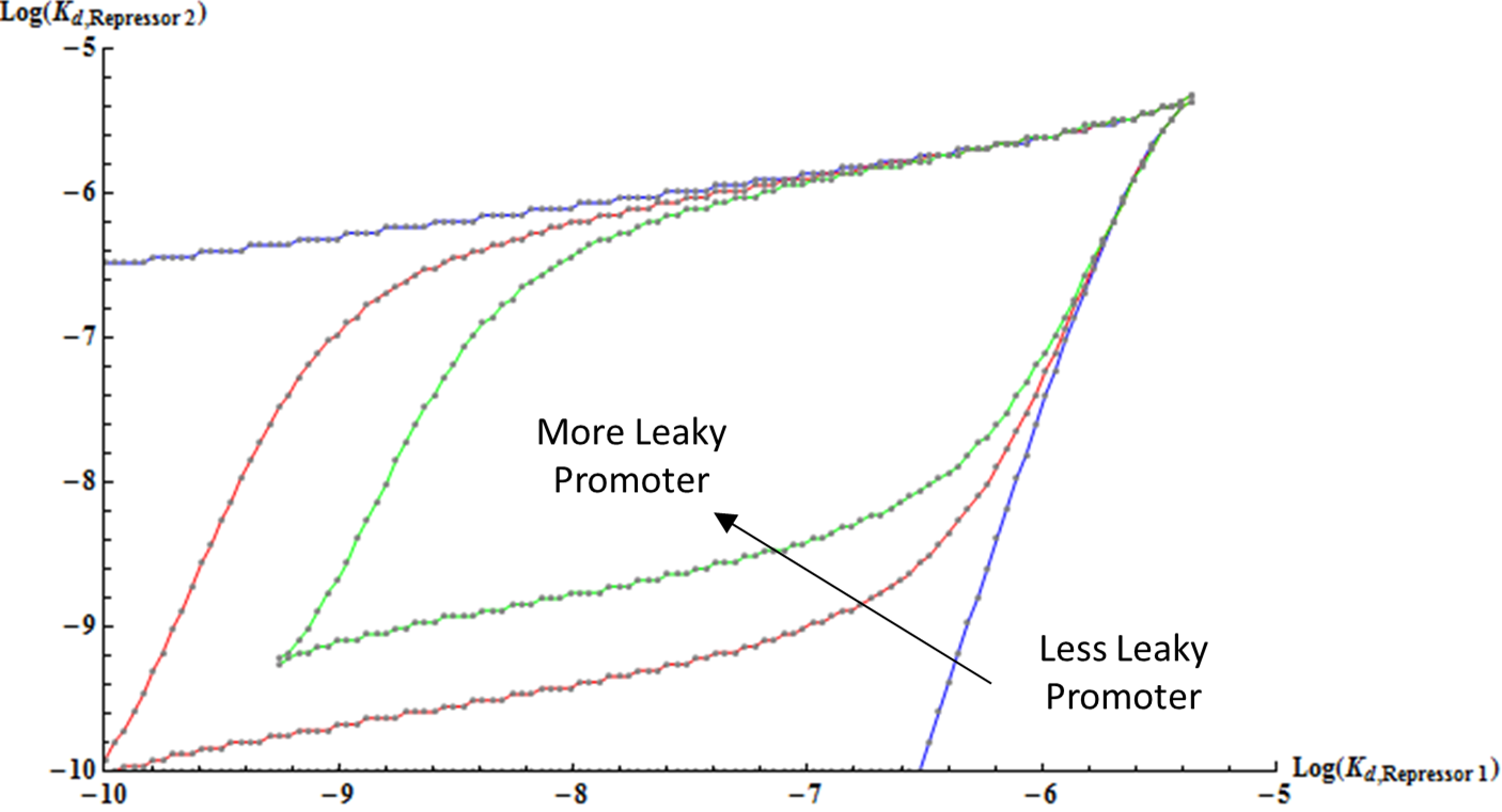
show graph
explain
show nullcline
confirm bistability of the system (thermodynamic model incorporated into kinetic model)
References
- Gardener, T. et al. Construction of a genetic toggle switch in Escherichia coli. Nature. 403, 339-342 (2000).
 "
"


