Team:Evry/Programming
From 2013.igem.org
| (4 intermediate revisions not shown) | |||
| Line 22: | Line 22: | ||
To solve our ODEs, we used a simple Euler method. Here is an example:<br/> | To solve our ODEs, we used a simple Euler method. Here is an example:<br/> | ||
Let the following be a Cauchy problem:<br/> | Let the following be a Cauchy problem:<br/> | ||
| - | <img src=""/><br/> | + | <img src="https://static.igem.org/mediawiki/2013/9/9b/Pro1.png"/><br/> |
Considering the following Taylor expansion:<br/> | Considering the following Taylor expansion:<br/> | ||
| - | <img src=""/><br/> | + | <img src="https://static.igem.org/mediawiki/2013/1/13/Pro2.png"/><br/> |
| - | + | <img src="https://static.igem.org/mediawiki/2013/c/c2/Pro3.png"/><br/> | |
| - | + | Let us define the sequence <img src="https://static.igem.org/mediawiki/2013/1/19/Pro4.png"/> such as <img src="https://static.igem.org/mediawiki/2013/9/9e/Pro5.png"/> and <img src="https://static.igem.org/mediawiki/2013/0/0c/Pro6.png"/><br> | |
| + | And thus, the sequence <img src="https://static.igem.org/mediawiki/2013/f/f1/Pro7.png"/> such as <img src="https://static.igem.org/mediawiki/2013/d/dc/Pro8.png"/> and <img src="https://static.igem.org/mediawiki/2013/9/9d/Pro9.png"/><br/> | ||
Thus, we can define the Euler method:<br/> | Thus, we can define the Euler method:<br/> | ||
| - | <img src=""/><br/> | + | <img src="https://static.igem.org/mediawiki/2013/4/4f/Pro10.png"/><br/> |
| - | Which, standardized, becomes <img src=""/>. | + | Which, standardized, becomes <img src="https://static.igem.org/mediawiki/2013/b/b0/Pro11.png"/>. |
</p> | </p> | ||
<p> | <p> | ||
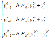
In the end, all our differential equation systems are implemented like so:<br/> | In the end, all our differential equation systems are implemented like so:<br/> | ||
| - | <img src=""/><br/> | + | <img src="https://static.igem.org/mediawiki/2013/d/d1/ProSystem.png"/><br/> |
where N is the number of equations in the system.<br/> | where N is the number of equations in the system.<br/> | ||
</p> | </p> | ||
| Line 41: | Line 42: | ||
</p> | </p> | ||
| - | <h2> | + | <h2>Flux Balance Analysis</h2> |
<p> | <p> | ||
| - | + | ||
| + | </p> | ||
| + | |||
| + | <h2>Cellular automaton</h2> | ||
| + | <p> | ||
| + | |||
</p> | </p> | ||
Latest revision as of 10:51, 26 October 2013
Programming methods
This part exposes our technical and algorithmical choices, the implementation and the numerical resolution of our models.
Models implementation
All our models are using the Python language. Python has several major perks:
- Very good floating numbers management
- High level programming
- Object-oriented
- Not an exclusively numerical tool, which allows much more options than Scilab or Matlab
Numerical resolution of ODEs
We chose not to use the resolution functions included in Scipy to have more coding liberties.
To solve our ODEs, we used a simple Euler method. Here is an example:
Let the following be a Cauchy problem:

Considering the following Taylor expansion:


Let us define the sequence  such as
  and
and 
And thus, the sequence  such as
  and
and 
Thus, we can define the Euler method:

Which, standardized, becomes  .
.
In the end, all our differential equation systems are implemented like so:

where N is the number of equations in the system.
This is how we implemented the equation systems in Python. The fact that we didn't use ODE-solving libraries allowed us to introduce definition domains for some variables, which improved the overall stability in numerical resolutions.
For a simpler and quicker use of repetitive tasks, we also encapsulated everything in a class scheme.
Flux Balance Analysis
Cellular automaton
 "
"


