Team:TU-Munich/Modeling/Enzyme
From 2013.igem.org
Introduction
To estimate the efficiency of our remediation rafts in detoxification of contaminated water, we saw the need to assess the activity of our target effectors. As in vivo experiments were still to be carried out we, started to analyse data we obtained in in vitro experiments.
We analysed the data for
| Experiment |
|---|
| [#Laccase (Substrate Dependence) Laccase (Substrate Dependence)] |
| Erethromycin esterase B (Substrate Dependence) |
| Laccase (pH Dependence) |
| Erethromycin esterase B (pH Dependence) |
| Laccase (NaCl Dependence) |
| Erethromycin esterase B (NaCl Dependence) |
Laccase (Substrate Dependence)
Data
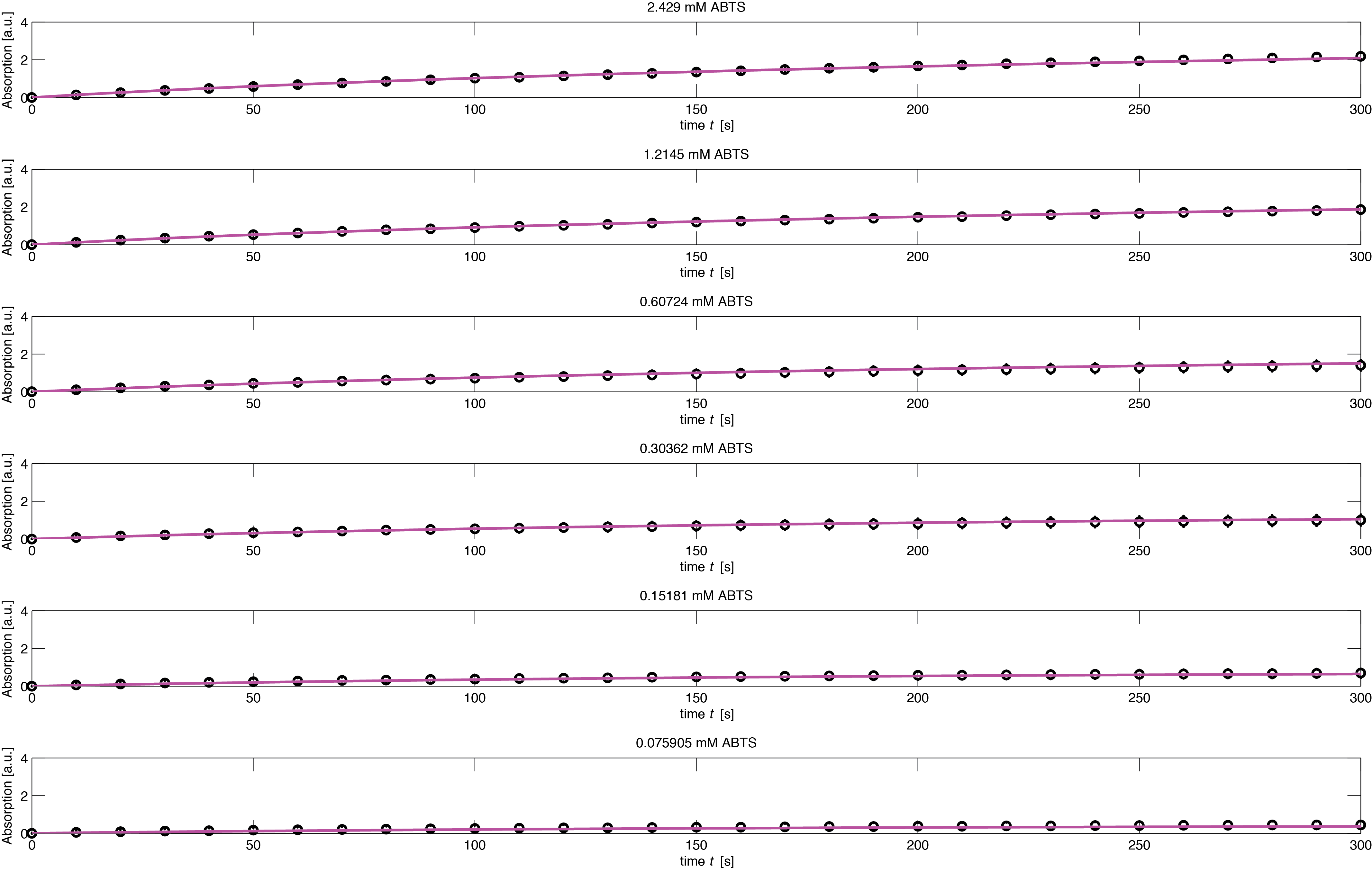
To assess the activity of <partinfo>BBa_K1159002</partinfo> we created an experimental setup with a dilution series for the concentration of the substrate ABTS with 16 different concentrations with a 2:1 dilution ratio resulting in concentrations ranging from 2.429 mM to 74.1 nM in triplicates and added 40.8 nM of purified enzyme. The concentration of the product of the enzymatic reaction was measured via absorption over 5 minutes with time steps of 10 seconds. As absorption measurements for very low substrate concentrations were almost undistinguishable from noise, we decided only to fit the data for the 8 highest concentrations. The data for the 8 highest concentration including standard deviation is shown in Figure 1.
Model
Calibration Curve
For quantitative modelling it is essential to relate the measured absorption with the concentration of the product of the enzymatic reaction. After initial investigation of the data we realised that the ratio between the absorption in the steady states was not scaling linearly with the dilution ratios. This led us to the conclusion that there was a nonlinear relationship between the concentration of the product of the enzymatic reaction and the absorption. Hence we contacted the wetlab and they measured a calibration curve for us such that we could carry out rigorous quantitative modeling.
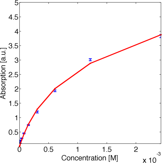
To use this curve later for modelling we fitted a parametric logarithmic curve in accordance with the [http://en.wikipedia.org/wiki/Beer–Lambert_law Beer-Lambert law]
by minimizing the corresponding log-likelihood assuming a normally distributed error. The obtained data and the corresponding fitted logarithmic curve are shown in figure 2, the resulting best fitting parameters are shown in table 1.
| Parameter | Best Fit |
|---|---|
| k1 | 1.651 a.u. |
| k2 | 3891 1/M |
Model Specification
For the Laccase kinetics we used the standard model for enzyme kinetics in reduced form.
We assumed a normally distributed measurement error which yielded us the following negative log likelihood
where ![]() is the mean of the experimental measurements at time point ti for the j-th experiment in the dilution series, σij denotes the corresponding standard deviation and yj is the numerical simulation of system Θ1 for parameters θ = [kf, kr, kcat] with the calibration curve applied to the output P at time ti.
is the mean of the experimental measurements at time point ti for the j-th experiment in the dilution series, σij denotes the corresponding standard deviation and yj is the numerical simulation of system Θ1 for parameters θ = [kf, kr, kcat] with the calibration curve applied to the output P at time ti.
Fitting
To obtain the best fitting parameters we used a multistart optimization in logarithmic parameter space with latin hypercube sampling as initialisation. Multistart optimization is employed to be sure that the resulting best fit is not a local optimum but a global one and logarithmisation of the parameter space is well-known to yield better results http://www.plosone.org/article/info:doi/10.1371/journal.pone.0074335 Raue et al., 2013. The parameter boundaries for the hypercube are shown in table 2.
| Parameter | Lower Bound | Upper Bound |
|---|---|---|
| kf | 1E+03 1/s | 1E+07 1/s |
| kr | 1E-05 1/s | 1E+06 1/s |
| kcat | 1E+00 1/s | 1E+08 1/s |
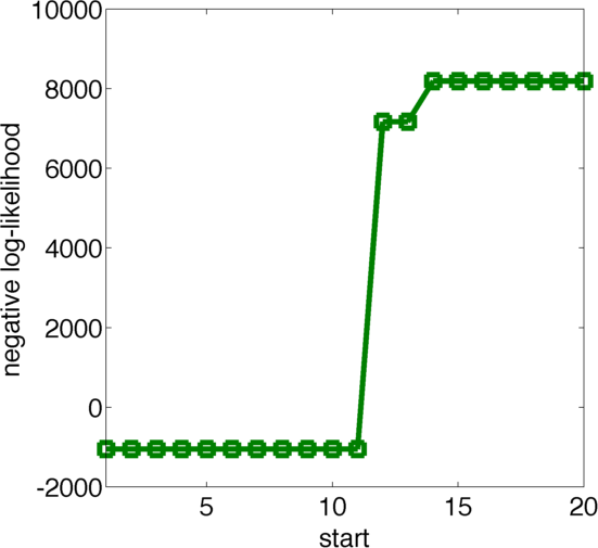
We used 20 initialisations for the multistart. Figure 4 shows the final value for the optimization routine for the different initial values, sorted by the resulting final value. As one can see there are 11 initialisations that yield approximately the same final result, which suggests that this might be a global optimum. Figure 3 displays the obtained parameters of the best fits colored according to their likelihood, where black is more likely and white is less likely.
These results suggest that parameter 3 (kcat) is very well identifiable, as all optimization runs yielded approximately the same parameter value. In contrast, the estimation of the two other parameters show strong uncertainties as the different initialisations yielded a range of different parameter values. Using the obtained parameters we can also compute KM which is used when Michaelis-Menten kinetics are assumed. The formula for this is
The obtained parameters for the best fit are shown in Table 3:
| Parameter | Best fit |
|---|---|
| kf | 4.196 E+06 1/s |
| kr | 1.399 E+03 1/s |
| kcat | 61.892 1/s |
| KM | 33.447 μM |
The simulation of the resulting parameter compared against the experimental data is shown in Figure 5.
These results suggest that we have obtained a reliable estimate for some of the parameter values and that the model seems sufficient to explain the experimental data. As there seems to be a certain uncertainty with respect to some of the parameters, we decided to carry out further uncertainty analysis to asses the reliability of the parameter estimates.
Uncertainty Analysis
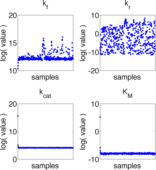
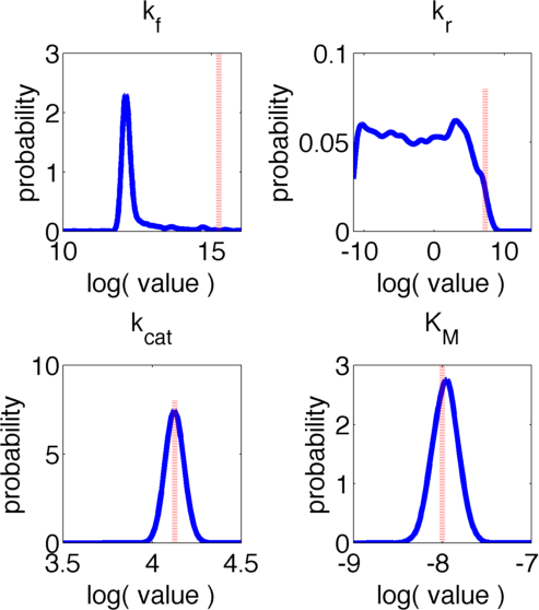
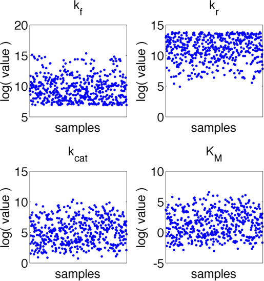
The uncertainties in measurement can be directly transferred into uncertainties in the parameter estimation with the help of the likelihood function. As the computation of the likelihood includes solving a non-trivial differential equation it is not possible to write down an analytical expression for it that could be used to estimate the parameter distributions. Hence we will have to resort to sampling from the parameter distribution. We did this using the Metropolis-Hastings algorithm implemented in the adaptive MCMC toolbox DRAM http://helios.fmi.fi/~lainema/mcmc/ Haario et al. (2006).We used a burn-in of 1,000 samples and then generated 400,000 samples from the distribution. Using these samples we can also generate samples for the parameter KM by computing KM for every sample via the same formula that was used above. For visualization 500 samples out of these 200,000 are shown in Figure 6. Using these samples we used standard kernel density estimation to estimate the marginal densities of single parameters. The resulting approximate marginal distributions are shown in Figure 7.
In Figure 6 and 7 one can see that all parameters except kr have localized parameter ranges of high probability, which means that we can expect our optimization should yield good results. Figure 7 shows the marginal densities of the parameters, obtained via kernel density estimation using MCMC samples, with the best parameter fits, obtained via optimization, indicated by red lines. As one can see, all fitted parameter except for kf are located in regions of high probability density.
We can explain this phenomenom by looking at the correlation between parameters. The correlation matrix of the parameter samples obtained via MCMC is presented in Table 4:
| kf | kr | kcat | |
|---|---|---|---|
| kf | 1 | 0.698 | -0.054 |
| kr | 0.698 | 1 | 0.027 |
| kcat | -0.054 | 0.027 | 1 |
Investigating the values presented in Table 4 one can see that there is a high correlation between parameters kf and kcat. The joint distribution of the samples in their values for kf and kr is shown in Figure 8. The likelihood of the individual samples is indicated by color. The best fit parameters are again displayed via a red dotted line. One can clearly see that there is a strong nonlinear correlation between the two parameters. Moreover it is evident, that despite having a low marginal likelihood for the obtained value of kf, in the joint distribution the best fit lies in a strongly localised area and we can accept the results with high certainty.
Erythromycin Esterase B (Substrate Dependence)
Data
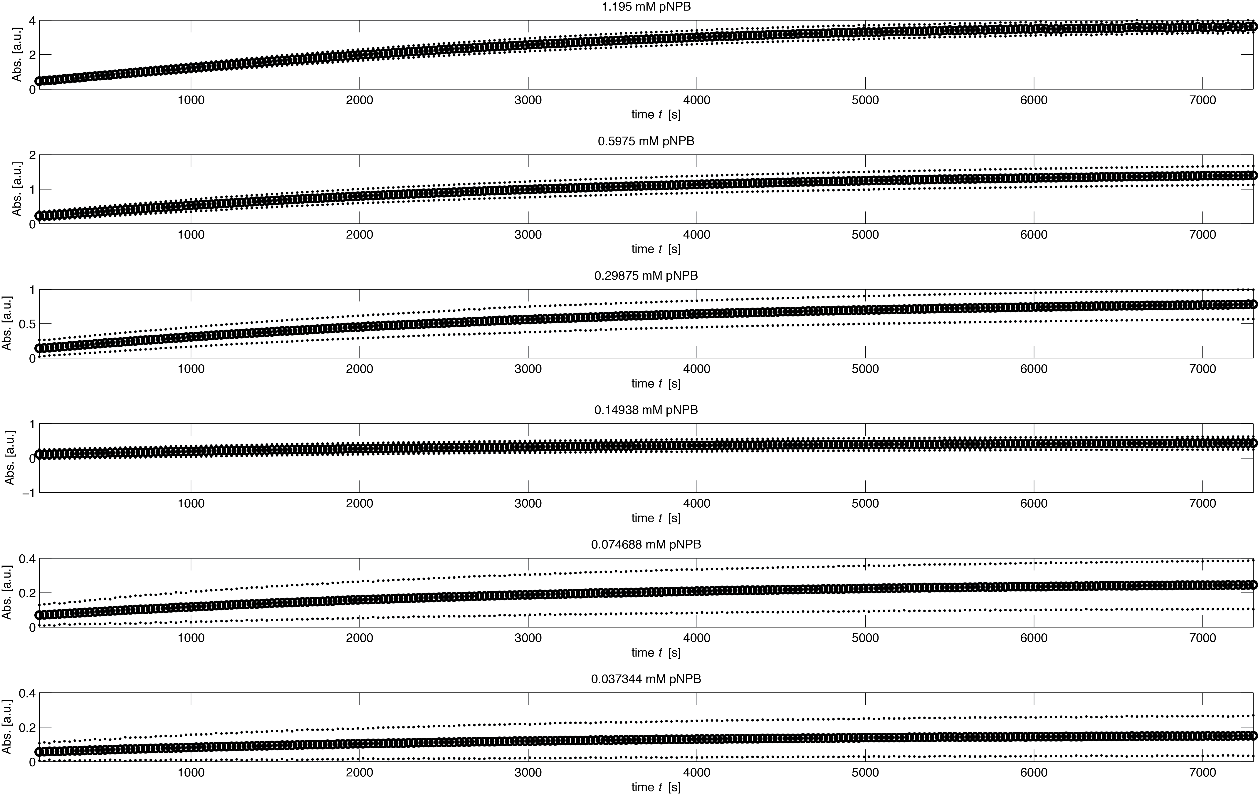
To assess the activity of <partinfo>BBa_K1159000</partinfo> we created an experimental setup with a dilution series for the concentration of the substrate p-NPB with 16 different concentrations with 2:1 dilution ratio resulting in concentrations ranging from 1.195 mM to 36.469 nM in triplicates and added 5.804 μM of purified enzyme. The concentration of the product of the enzymatic reaction was measured via absorption for the duration of 2 hours with a time steps of 30 seconds. As measurements for very low substrate concentrations were almost undistinguishable from noise, we decided only to fit the data for the 6 highest concentrations.
Model
Calibration Curve
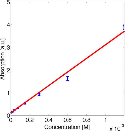
For quantitative modelling it is essential to set the measured absorption into relationship with the concentration of the product of the enzymatic reaction. For this experimental setup we saw that there was a purely linear relationship between concentration and absorption. Hence we found it sufficient to fit a linear curve to the measured absorption of reference concentrations by minimizing the corresponding log-likelihood assuming a normally distributed error. The best fitting parameters are shown in table 5. The formula for the linear curve was
| Parameter | Best Fit |
|---|---|
| k1 | 3.005 E+03 a.u./M |
| k2 | 0.118 a.u. |
Substrate Auto-degradation
In the negative control for the experiment, where no enzyme was added, we noticed that there was an noticeable autocatalytic degradation of the substrate for sufficiently high substrate concentrations. As this led to significant absorption levels without any enzyme present, we decided to fit this degradation rate and integrate it into our model. Moreover there was a timespan of about 300 seconds missing from the induction of the experiment until the beginning of the measurement. We also used the degradation to get a more reliable estimate of the time between induction and start of measurement.
Model Specification
For the EreB kinetics we used the standard model for enzyme kinetics in reduced form but added the autocatalytic degradation term γS.
We assumed a normally distributed measurement error which yielded us the following negative log likelihood
where ![]() is the mean of the experimental measurements at time point ti for the j-th experiment in the dilution series, σij denotes the corresponding standard deviation and yj is the numerical simulation of System1 for parameters theta = [kf, kr, kcat] with the calibration curve applied to the output P at time ti.
is the mean of the experimental measurements at time point ti for the j-th experiment in the dilution series, σij denotes the corresponding standard deviation and yj is the numerical simulation of System1 for parameters theta = [kf, kr, kcat] with the calibration curve applied to the output P at time ti.
Fitting
To obtain the best fitting parameters we used a multistart optimization in logarithmic parameter space with latin hypercube sampling as initialisation. Multistart optimization is employed to be sure that the resulting best fit is not a local optimum but a global one and logarithmisation of the parameter space is well-known to yield better results http://www.plosone.org/article/info:doi/10.1371/journal.pone.0074335 Raue et al., 2013. The parameter boundaries for the hyper cube are shown in table 6.
| Parameter | Lower Bound | Upper Bound |
|---|---|---|
| kf | 1E+00 1/s | 1E+10 1/s |
| kr | 1E-05 1/s | 1E+10 1/s |
| kcat | 1E+00 1/s | 1E+10 1/s |
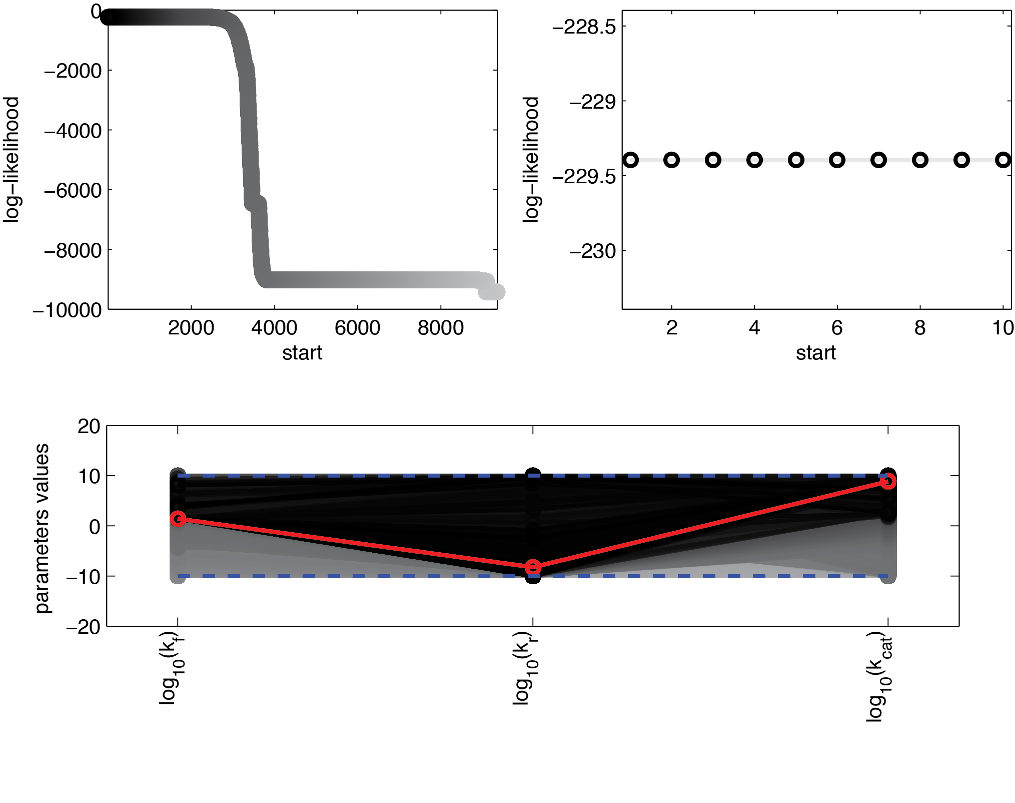
We used 20 initialisations for the multistart. Figure 13 shows the final value for the optimization routine for the different initial values, sorted by the resulting final value. As one can see there are 11 initialisations that yield approximately the same final result, which suggests that this might be a global optimum. Figure 12 displays the obtained parameters fo the best fits colored according to their likelihood, where black is more likely and white is less likely.
These results suggest that parameter 1 (kf) is relatively well identifiable, while the estimation of the two other parameters show strong uncertainties. Using the obtained parameters we can also compute KM which is used when Michaelis-Menten kinetics are assumed. The formula for this is
The obtained parameters for the best fit are shown in Table 7:
| Parameter | Best fit |
|---|---|
| kf | 43.233 1/s |
| kr | 2.804 1/s |
| kcat | 1.579 E+08 1/s |
| KM | 6.488 E+03 M |
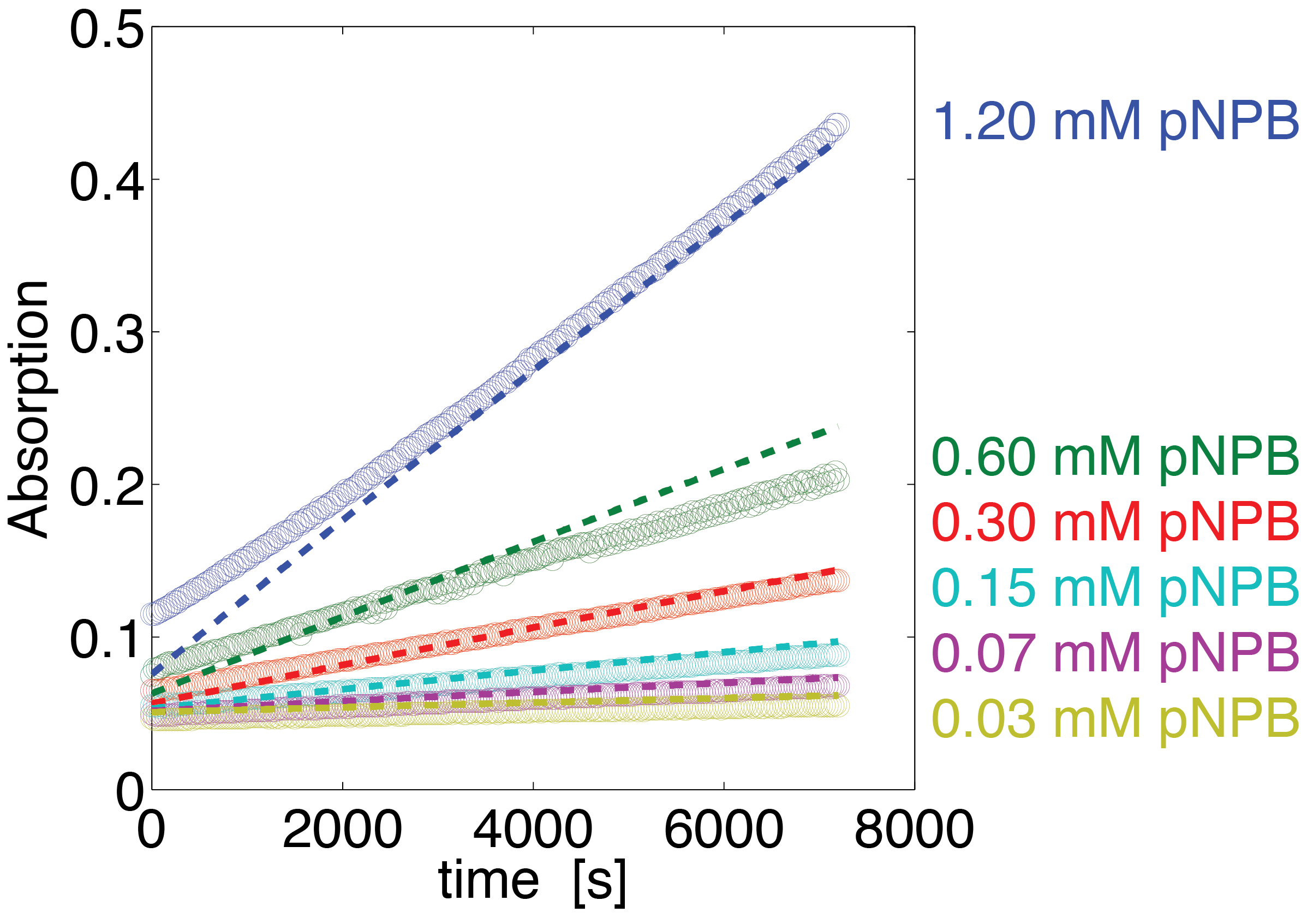
The simulation with the resulting parameter compared against the experimental data is shown in Figure 14.
Uncertainty Analysis
The uncertainties in measurement can be directly transferred into uncertainties in the parameter estimation with the help of the likelihood funtion. As the computation of the likelihood includes solving a non-trivial differential equation it is not possible to write down an analytical expression for it that could be used to estimate the parameter distributions. Hence we will have to resort to sampling from the parameter distribution. We did this using the Metropolis-Hastings algorithm implemented in the adaptive MCMC toolbox DRAM http://helios.fmi.fi/~lainema/mcmc/ Haario et al. (2006). We used a burn-in of 1,000 samples and then generated 400,000 samples from the distribution. Using these samples we can also generate samples for the parameter KM by computing KM for every sample via the same formula that was used above. As a visualization 500 samples out of those 200,000 are shown in Figure 15. Using these samples we used kernel density estimation to estimate the marginal densities of single parameters. The resulting approximate marginal distributions are shown in Figure 16.
As one can see in Figure 15 and 16 none of the parameters have localised parameter ranges of high probabilities, which means that we can expect them to perform badly. Moreover we see that the density rapidly drops at the boundaries of the investigated domain, which means that the domain boundaries were badly chosen. Due to the computational intensity of the uncertainty analysis we were not able to repeat this experiment, but this will be done after the Jamboree.
Comparision to Literature data
In a recent paper http://pubs.acs.org/doi/abs/10.1021/bi201790u?mi=0&af=R&pr... Wright et al., 2012 characterizing EreB the kinetic properties of EreB were also analyzed using p-NPB. However only kcat and KM were determined, the results of which are shown in table 8.
| literature values | our values | |
|---|---|---|
| KM | 1.7 E-03 M | 6.5 E+03 M |
| kcat | 2.8 E+00 1/s | 1.6 E+08 1/s |
| kcat/KM | 6.0 E+04 s-1 M-1 | 2.5 E+04 s-1 M-1 |
It can be seen that our estimates of KM and kcat diverge by several magnitudes from the values determined by the Wright group, however for the activity of the enzyme kcat/KM the difference is only a factor of 2. Since this is a key characteristic of an enzyme, which appears when further simplifying the Michaelis-Menten kinetics, the close correspondence here indicates a similarly active protein, supporting the results of our modeling.
Laccase (pH Dependence)
Erythromycin Esterase B (pH Dependence)
Laccase (NaCl Dependence)
Erythromycin Esterase B (NaCl Dependence)
MatLab Scripts
References:
http://helios.fmi.fi/~lainema/mcmc/ Haario et al. (2006) H. Haario, M. Laine, A. Mira and E. Saksman, (2006). DRAM: Efficient adaptive MCMC, Statistics and Computing 339-354(16).
http://www.plosone.org/article/info:doi/10.1371/journal.pone.0074335 Raue et al. (2013) A. Raue, M. Schilling, J. Bachmann, A. Matteson, M. Schelke, D. Kaschek, S. Hug, C. Kreutz, B. D. Harms, F. J. Theis, U. Klingmüller, J. Timmer (2013). Lessons Learned from Quantitative Dynamical Modeling in Systems Biology, PLOS ONE
http://pubs.acs.org/doi/abs/10.1021/bi201790u?mi=0&af=R&pr... Wright et al., 2012 Morar, M., Pengelly, K., Koteva, K. and Wright, D. (2012). Mechanism and Diversity of the Erythromycin Esterase Family of Enzymes. Biochemistry, 51(8): 1740–1751.
 "
"








AutoAnnotator:
Follow us:
Address:
iGEM Team TU-Munich
Emil-Erlenmeyer-Forum 5
85354 Freising, Germany
Email: igem@wzw.tum.de
Phone: +49 8161 71-4351