Team:TU-Munich/Modeling/Kill Switch
From 2013.igem.org
Kill Switch Modeling
Purpose
The idea of our kill switch is to kill off our moss, as soon as it leaves the filter system. For this purpose two methods were proposed:
- siRNA method: When some trigger is activated, siRNA is expressed inhibiting the expression of a vital gene
- nuclease method: When some trigger is activated, a nuclease is released destroying the DNA of the cell
To decide between these two methods we modelled the vitality V of the cell (a number between 0 and 1, so a perfectly functional cell has V=1, a dead cell V=0) and depending on the tested method the concentration of siRNA R and nuclease N as appropriate. Both concentrations are normalized to the unit interval [0,1].
siRNA Model
Governing equations
We determined the governing equations of this model to be the following:with initial conditions V(0) = 1 and R(0) = 0, where at the time t=0 the trigger is activated.
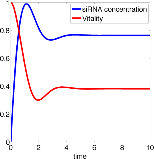
Figure 1, created by our MatLab script siRNA model shown below, on the right shows a solution to this system for some example parameters. In this case the vitality of the cell decreases to somewhere around 0.3 while at the same time after an initial peak the siRNA concentration also drops upon which the vitality settles in at about 0.4.
So it appears, that the siRNA approach does not achieve the required death of the cells. In the following it will be shown, that this is the case for all parameter values.
Calculation of stable points and analysis
The steady points V* and R* of this system have to satisfy Defining
If α = 1, the unique steady point is ![]() .
.
These are both negative, so this is a stable point, i.e. an attractor.
Now only one of these is in the sensible range, because
So there is only one steady point in this range, namely:
By expanding the fraction by ![]() we can rewrite V* as
we can rewrite V* as
So using the results from above, we get: ![]()
Defining ![]() , the eigenvalues are given by
, the eigenvalues are given by
So ![]() , which means that this is a stable attractor.
, which means that this is a stable attractor.
Result of our model
So for the siRNA there always is a stable point for the vitality between (but excluding) 0 and 1, so the moss is not killed-off completely, just impeded in its growth.
Interpretation
This result makes intuitive sense, because as the function of the cell is repressed the cell produces less of the inhibiting siRNA, which leads to a regeneration of the cell. Eventually a steady state at a lower vitality is reached, where the vitality stays constant.
Nuclease Model
Governing equations
We determined the governing equations of this model to be the following:with initial conditions V(0) = 1 and N(0) = 0, where at the time t=0 the trigger is activated.
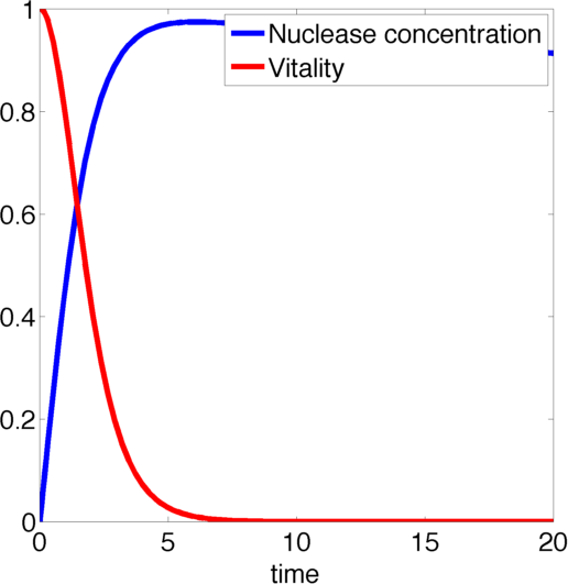
Figure 2, created by our MatLab script nuclease model shown below, on the left shows a solution to this system for some example parameters. It clearly shows that in this case the vitality of the cell decreases to 0 and remains there, i.e. that the cell has died.
In the following we will verify, that this is the case for all parameter values.
Calculation of stable points and analysis
Any steady state given by V* and N* of this system must to satisfy
The eigenvector corresponding to the zero eigenvalue is ![]() . It is obvious from the equations that any disturbance away from the steady state along this vector will decay back to the steady state, so this is a stable attractor.
. It is obvious from the equations that any disturbance away from the steady state along this vector will decay back to the steady state, so this is a stable attractor.
Results of our model
The nuclease always reduces the vitality of the moss to 0, i.e. kills it off completely.
Interpretation
Again this result is very intuitive, since the moss cannot regenerate from the destruction of its genome.
Conclusions
For a functional kill-switch it is necessary, that the cells are actually killed and not just live on with reduced vitality. So based on our modeling results the siRNA approach is not satisfactory, while the nuclease satisfies the requirement. As a result the team pursued the nuclease approach leading to our final kill-switch.
MatLab Scripts
siRNA model script
% f = @(R,V,k) [k(3)* V  - k(4) * R , -k(1) * R * V + k(2) *(V  -1)* (R  -1)];
g = @(k,y)    [k(3)* y(2)- k(4)*y(1); -k(1)*y(1)*y(2)+k(2)*(y(2)-1)*(y(1)-1)];

%k= [  k1,  k2,  k3,  k4 ]; %insert the appropriate reaction rate constant
k = [   1,   2,   2,   1];

[TOUT, YOUT] = ode45(@(t,y) g(k,y) ,[0,10],[0;1]);

plot(TOUT, YOUT(:,1), 'markersize', 15, 'linewidth', 5)
hold on; plot(TOUT, YOUT(:,2), 'r', 'markersize', 15, 'linewidth', 5); hold off

legend('siRNA concentration','Vitality');
xlabel('time');
set(gca,'FontSize',24);
set(gcf,'position', [100 100 600 600]);

axis square
set(gcf,'Color','w');
export_fig siRNA_pic.png
nuclease model script
% f = @(N,V,k) [p(3)* V  - p(4) * N , -p(1) * N * V  ];
g = @(p,y)    [p(3)* y(2)- p(4)*y(1); -p(1)*y(1)*y(2)];

%p= [  p1,  p2,  p3,  p4 ]; %insert the appropriate reaction rate constant
p = [   1, NaN,   1, 0.5 ];

[TOUT, YOUT] = ode45(@(t,y) g(p,y) ,[0,20],[0;1]);

plot(TOUT, YOUT(:,1), 'markersize', 15, 'linewidth', 5)
hold on; plot(TOUT, YOUT(:,2), 'r', 'markersize', 15, 'linewidth', 5); hold off

legend('Nuclease concentration','Vitality')
xlabel('time');
set(gca,'FontSize',24);
set(gcf,'position', [100 100 600 600]);

axis square
set(gcf,'Color','w')
export_fig nuc_pic.png
 "
"


AutoAnnotator:
Follow us:
Address:
iGEM Team TU-Munich
Emil-Erlenmeyer-Forum 5
85354 Freising, Germany
Email: igem@wzw.tum.de
Phone: +49 8161 71-4351