 "
"
Team:British Columbia/Modeling
From 2013.igem.org
AnnaMüller (Talk | contribs) (→References) |
Joelkumlin (Talk | contribs) |
||
| Line 223: | Line 223: | ||
Where $V$ is the volume of the bioreactor ($L$), $\frac{dS}{dt} is the substrate utilization rate ($in g L^{-1} s^{-1}$),$F$ is the flow rate in ($L h^{-1}$), $\mu$ is is the growth rate ($h^{-1}$), $Y_{X/S}$ is the yield coefficient of biomass with respect to substrate, $q_p$ is the specific oxygen uptake rate ($hr^{-1}$). | Where $V$ is the volume of the bioreactor ($L$), $\frac{dS}{dt} is the substrate utilization rate ($in g L^{-1} s^{-1}$),$F$ is the flow rate in ($L h^{-1}$), $\mu$ is is the growth rate ($h^{-1}$), $Y_{X/S}$ is the yield coefficient of biomass with respect to substrate, $q_p$ is the specific oxygen uptake rate ($hr^{-1}$). | ||
| - | Using | + | Using equations in the mono-culture growth section we model start up of the bioreactor in both lag and batch phases. Once the fed batch phase begins we use the growth equation: |
| + | |||
| + | \begin{align} | ||
| + | \frac{dX}{dt} &= X\big(\mu - \frac{F}{V}\big)\\ \ \\ | ||
| + | \frac{F}{V} &= \frac{\mu X}{Y_{X/S} \Delta S} | ||
| + | \end{align} | ||
| + | |||
| + | |||
| + | |||
== References== | == References== | ||
Revision as of 23:56, 27 October 2013
iGEM Home


Population Dynamics Modeling
Mixed cultures are often used in bioprocessing, where the quality of the final product requires optimal strain balance. We realized that mixed cultures harbouring different CRISPR assemblies could be modulated by applying selective pressure against targeted strains via phage addition. This provides a novel opportunity for tuning bacterial consortia, directly applicable to industrial bioprocesses such as yogurt production that rely on mixed culture fermentation. Here, we develop analytical and numerical models to provide a predictive framework for optimizing strain balance within mixed populations. We then extend this model to allow for optimization of product formation, such as flavouring of yogurt.
Our main objectives were as follows:
- Predict the growth of recombinant E. coli cultures under phage predation.
- Predict caffeine production based on initial number of viruses, (ie. multiplicity of infection; MOI).
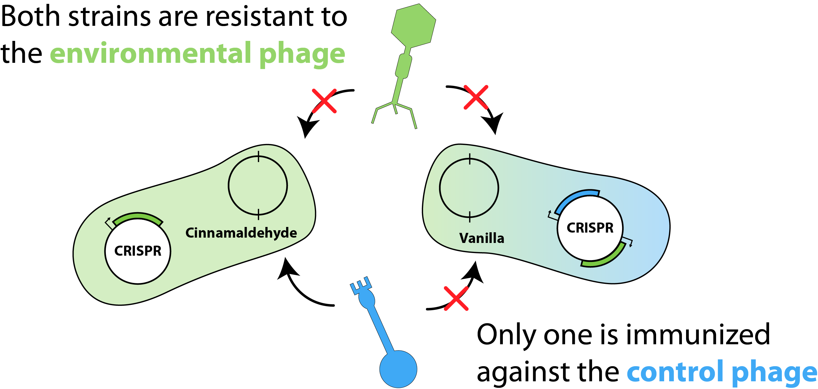
To help conceptualize our model, we first generated the schematic shown in Figure 1. For simplicity, we considered two e.coli strains each harbouring two plasmids: a flavouring plasmid and a CRISPR (or "immunity") plasmid. Here, the flavouring plasmid is responsible for the production of either cinnamaldehyde or vanillin and the CRISPR plasmid contains unique spacer elements, granting the strain immunity against "environmental phage" that may contaminate the bioreactor. Additionally, one strain would be immunized against the "control phage" allowing us to modulate the population with phage targeting the un-immunized strain.
Modeling bacteria growth under phage predation
An analytical model based on Monod kinetics [1] was used to describe bacterial growth. Here, the Poisson distribution was incorporated to model the infected populations based on a starting phage-to-bacteria ratio, or MOI. We trained the model on a set of experimental growth curves and validated it against a separate set. Yield terms were added to account for the production of two different flavours: cinnamaldehyde and vanillin. Next, we extended our basic growth model to include bacterial co-cultures. Using this approach, we demonstrate that by using different virus inoculums, it is possible to achieve different final amounts of compounds from a mixed culture.
Simulating virus-mediated population control
To simulate the behaviour of cells growing in mixed populations, we numerically modeled the co-cultures of two flavouring product strains using the cell programming language "gro" [2]. The model considers two strains of bacteria on a two-dimensional surface under phage predation. One of the strains is immune to infection, whereas the other is susceptible.
Model Formulation
Assumptions
- Bacteria is grown in a batch culture and follows the Monod growth equation.
- Bacteria with the CRISPR are nearly 100% immune to the specific phage infection.
- Bacteria without CRISPR system are completely susceptible to phage infection.
- Yield coefficients and phage attachment coefficients are constants.
- Bacterial phages do not decrease significantly in number during the course of an experiment.
- All considered bacterial phages are lytic.
Analytical Model
Bacteria Growth
We begin with a populations balance for a given strain $X$, \begin{align} \frac{dX}{dt} = \frac{dX_i}{dt} + \frac{dX_u}{dt} \end{align} The infected bacteria is represented by $X_i$, uninfected bacteria by $X_u$ and $X = X_i + X_u$. We use the Monod equation to model the substrate limited bacterial growth. \begin{align} \mu_{X} = \mu_{max, X} \frac{S}{K_{S, X} + S} \end{align}
Where $\mu_{X}$ is the bacterial growth rate, $\mu_{max, X}$ is the maximum bacterial growth rate, $S$ is the growth limiting substrate and $K_s$ is the amount of substrate remaining when the growth rate is half of maximum. Due to environmental factors, some bacteria will die; the death rate ($k_d$) is assumed to be directly proportional to the bacteria population. A lag phase is modelled by multiplying a dampening term to the growth rate, namely $(1 - e^{-\alpha t})$, where $\alpha$ is defined as a proportionality constant. The slowing of growth from exponential to stationary is modelled with yet another dampening term to be multiplied to the growth: $exp\big[{-\big(\frac{X}{X_c}\big)^m\big]}$. This dampening term is related to the quorom sensing in bacteria, once the bacteria reach some characteristic concentration ($X_c$) the bacteria begin to slow down growth. Thus the uninfected cell growth is described by: \begin{align} \frac{dX_u}{dt} = \big( \mu_{X, u}e^{-\big(\frac{X}{X_c}\big)^m} - k_{d_{X,u}} \big) X_u\big(1 - e^{-\alpha t}\big) \end{align} For simplicity, in this model, $m$, $X_c$, and $\alpha$ are all to be empirically determined and assumed constant. In reality, each constant is dependent on many variables, for example: $\alpha(temperature, pressure, [substrate], environmental \ conditions, bacterial \ strain, more)$. Similarly for infected cells: \begin{align} \frac{dX_i}{dt} = \big( \mu_{X, i}e^{-\big(\frac{X}{X_c}\big)^m} - k_{d_{X,i}} \big) X_i\big(1 - e^{-\alpha t}\big) - \delta \end{align}
However, a major difference is that the decay rate for the infected cells is dependent on the latency time of the virus and thus we introduce $\delta$. The function $\delta$ is defined as follows,
Here $N(\tau)$ is a normal distribution over some time $\tau$, in other words, it is expected that the infected population will lyse according to a normal distribution over the domain $(-\tau, \tau)$.
Viral Growth
It is now necessary to consider the phage population $V$ as it directly affects the amount of bacteria that are infected at any given time. To describe the phage population it is necessary to consider how many phages are released per cell lysis, this number is referred to as the burst size $(\beta)$. \begin{align} V = V_0 + X_i \beta ^{\frac{t}{LT}} \end{align} Where $V_0$ is the initial phage populations and $LT$ is the latency time (they time between infection and lysis). However, since lab techniques are tricky to measure the exact phage at various time points as well as the exact amount of infected bacteria, it is desired to simplify the model. It is reasonable to use a stepwise function that describes the amount of free phage present. Also, since the burst size is large, on the order of $100$ [3], we see that the loss of current phage due to infection of cells is small (roughly 1%), thus to simplify computations we consider this to be negligible. With these deductions we arrive at the following: \begin{align} V = V_0 + E(X_i)\beta^{\big[\frac{t}{LT}\big]} \end{align} Where $E(X_i)$ is the expected infected population and $\big[\frac{t}{LT}\big]$ is the largest integer equal or less than $\frac{t}{LT}$. To find the expected infected population, the Poisson distribution is used based on the MOI. However, there is an efficiency of viral attachment $\epsilon \in (0, 1)$ (in fact the efficiency has been found to be a function of certain proteins) [4,5]. \begin{align} MOI = \frac{V}{X} \end{align}
\begin{align} E(X_i) = \epsilon X(1 - e^{-MOI}) \end{align}
Substrate Utilization
The bacteria will need to use a substrate, and the depletion of this substrate is proportional to the growth of the uninfected bacteria and the amount of bacteria. Although the infected bacteria do not multiply when infected, the infected cells may use up substrate to gain the energy needed to replicate the phage. Although it may be the case that the bacteria simply recycle intracellular material, a substrate utilization term ($\gamma$) for the infected cells is utilized (if the bacteria do in fact recycle intracellular material, it follows that this value will be 0). Moreover, when cells lyse, the cell materials can be metabolized by other bacteria and will add to the amount of nutrients available. Thus, the equation for substrate utilization rate is:
\begin{align} \frac{dS}{dt} = - \big[ \frac{\mu_u}{Y_u}X_u + \frac{\gamma}{Y_i}X_i \big] + \phi \delta \end{align} Where $Y_u$ and $Y_i$ are yield constants and $\phi$ is the average amount of substrate released per infected cell during lysis. For clarity, $\delta$ is as described above.
Model Validation
Although, only limited amounts of growth curves have been able to be analyzed, the initial quantitative results appear promising and the qualitative results have been found to contain information whether or not the quantitative results align. The qualitative curve were especially good at predicting culture collapse (keep in mind that OD measurements will contain "bacterial bones" which will artificially inflate the concentration of bacteria after lysis).

Figure 1 - Bacteria Growth curves from lag phase to approaching stationary phase. The model was optimized on another set of data and was tested for validity on this set.

Figure 2 - Bacteria Growth under phage predation. In models where the quantitative values differ, there is still qualitative information that can be extracted.

Figure 3 - A better fit for bacteria Growth under phage predation. Also included, the predicted infected and uninfected populations.
Product Formation
For a given uninfected bacteria $X_u$ that can produce the product $P$, we will first expect the production rate to be first order equation: \begin{align} \frac{d[P]}{dt} = \frac{\mu_{X_u}}{Y_P}X_u \end{align} Where $Y_P$ is the yield coefficient of the product. For infected bacteria we expect the product formation rate to be negligibly small.
Extending to Co-culture
The end goal of our project is to tune product formation by adding phage to a batch reactor at the same time as having one flavour in constant production. Thus, we must model a two culture system. Let our bacterial cultures be called $X$ and $Z$. Let Z be immunized to the phage with our CRISPR system. Our equations become:
Subject to initial and boundary conditions:
We used Matlab to solve the system of equations and we plot the resulting product formations over time with different initial MOI's.

Figure 4 - Theoretical product formations based on co-culture dynamics. The thicker lines depict a higher MOI than the thinner lines.
Numerical Model
For the numerical simulation of co-cultures we utilized the cell programming language gro, developed by the Klavins Lab at the University of Washington [2]. The model considers two strains of bacteria on a two dimensional plane under attack of one virus. One strain has the CRISPR element and is immune to infection whereas the other is susceptible. In the simulation, susceptible bacteria entering regions with high phage concentrations are very likely to become infected and upon lysis increase the phage concentration of that region.

Bioreactor Design
Bioreactors are a specialized type of reactor that use cells to produce products of interest, and have become a ubiquitous tool in the bioprocess industry [1]. We wanted to apply our model to a more industrially applicable situation. The goal of this design is to produce 1,500 kg/year of cinnamaldehyde throughout the course of 320 operational days, operating 24 hours a day and 7 days a week. The growth rate of E.coli Additionally, each fermentation cycle would be composed of 5 phases: lag (no cell growth or product production), batch (constant volume, no inflow of substrate), fed-batch (introduction of glucose feed to keep substrate concentration constant), continuous (equal flow into and out of the reactor keeping volume, and constant substrate concentration), and production phase (product production, with negligible growth rate).
The fermenter itself was kept at 30 ˚C, pH 6.8 (via alkaline buffer control), and the following assumptions were made: negligible cell death, sterile substrate feed, well-mixed reactor, foam level controlled automatically and does not affect liquid volume, product production only after induction, tank is aluminum oxide, requires added cooling jacket and coil system, and negligible heat loss to the surroundings. Moreover, glucose was used at the substrate of choice (300 g/L feed solution). At maximum cell density the heat load was 3,684,983 kJ/h, which required an internal cooling coil length of 997 m, with a 12 ˚C water flow rate of 5105.98 and 35388.15 L/hr for the jacket and internal coils respectively. The reactor has a volume of 16.7 m3, a diameter of 1.78 m, and a pressure of 1 atm. 4 Rushton impellers are utilized. The kLa determined for this fermentation process is 1974.36 hr-1.
The biomass and substrate utilization equations were derived, using the following overall mass balance equation for the reactor system: \begin{align} V \frac{dS}{dt} = FS_0 - FS - V \mu X \frac{1}{Y_{X/S}} - Vq_pX\frac{1}{Y_{X/S}} \end{align}
Where $V$ is the volume of the bioreactor ($L$), $\frac{dS}{dt} is the substrate utilization rate ($in g L^{-1} s^{-1}$),$F$ is the flow rate in ($L h^{-1}$), $\mu$ is is the growth rate ($h^{-1}$), $Y_{X/S}$ is the yield coefficient of biomass with respect to substrate, $q_p$ is the specific oxygen uptake rate ($hr^{-1}$).
Using equations in the mono-culture growth section we model start up of the bioreactor in both lag and batch phases. Once the fed batch phase begins we use the growth equation:
\begin{align} \frac{dX}{dt} &= X\big(\mu - \frac{F}{V}\big)\\ \ \\ \frac{F}{V} &= \frac{\mu X}{Y_{X/S} \Delta S} \end{align}
References
[1] Shuler, M.L. & Kargi, F. (2002). Bioprocess Engineering: Basic Concepts (2nd ed.). Prentice Hall, Upper Saddle River, NJ.
[2] Jang, S.S., Oishi, K.T., Egbert, R.G., & Klavins, E. (2012). Specification and simulation of multicelled behaviors. ACS Synthetic Biology 1 (8), pp 365–374.
[3] Simon, E. H., Tessman, I. (1963). Thymidine-requiring Mutants of Phage T4. PNAS, 50, 526–532.
[4] Storms, Z. J., Arsenault, E., Sauvageau, D., & Cooper, D. G. (2010). Bacteriophage adsorption efficiency and its effect on amplification. Bioprocess and Biosystems Engineering, 33(7), 823–31.
[5] Storms, Z. J., Smith, L., Sauvageau, D., & Cooper, D. G. (2012). Modeling bacteriophage attachment using adsorption efficiency. Biochemical Engineering Journal, 64, 22–29.