"
"
Team:Evry/Modelmeta1
From 2013.igem.org
| (31 intermediate revisions not shown) | |||
| Line 9: | Line 9: | ||
<h2>Introduction</h2> | <h2>Introduction</h2> | ||
<p> | <p> | ||
| - | In order to determine our | + | In order to determine our <b><span style="color:#bb8900">Iron</span><span style="color:#7B0000"> Coli</span></b>'s enterobactin production rate, we first have to know how much time our bacteria will take to sense the ambient iron. So, this first part of the <i>Enterobactin production model</i> focuses on the synthetic <a href="https://2013.igem.org/Team:Evry/Sensor">sensing system</a> our team implemented in the bacteria. |
</p> | </p> | ||
<h2>Observations</h2> | <h2>Observations</h2> | ||
<p> | <p> | ||
| - | As shown on the <a href="#Fig1">Figure 1</a>, our sensing system relies on a | + | Naturally, when there is a large amount of iron in the environment, 2 iron ions complex with 2 <a href="https://2013.igem.org/Team:Evry/FUR_Project">FUR</a> proteins and bind to the FUR Binding Site (FBS). This interaction regulate negativelly the genes downstream. <br/> |
| + | As shown on the <a href="#Fig1">Figure 1</a>, our sensing system relies on a FBS. In order to easily model the sensing delay and analyse its results, the first construction is composed of a GFP placed right after the FBS. | ||
| + | |||
</p> | </p> | ||
| - | <div class="captionedPicture" style=" | + | |
| - | <a title="Nom Lien" href="https://static.igem.org/mediawiki/2013/ | + | |
| - | <img alt="Nom Lien" src="https://static.igem.org/mediawiki/2013/ | + | <div align="center"> |
| + | <a id="Fig1"></a> | ||
| + | <div class="captionedPicture" style="width:60%;"> | ||
| + | <a title="Nom Lien" href="https://static.igem.org/mediawiki/2013/4/47/ModelFurGfp.png"> | ||
| + | <img alt="Nom Lien" src="https://static.igem.org/mediawiki/2013/4/47/ModelFurGfp.png" width="50%" alt="First construction" class="Picture"/> | ||
</a> | </a> | ||
<div class="caption"> | <div class="caption"> | ||
| - | <b>Figure 1:</b> <p> | + | <b>Figure 1:</b> Our first construction, our Iron sensor system<p> |
| + | See <a href="https://2013.igem.org/Team:Evry/Sensor" target="_blank">our sensor page</a> for more details</p> | ||
</div> | </div> | ||
</div> | </div> | ||
| - | + | <div style="clear: both;"> | |
| - | <div style="clear: both;"></div> | + | </div></div> |
<h2>Goals</h2> | <h2>Goals</h2> | ||
| Line 33: | Line 40: | ||
<ul> | <ul> | ||
<li>We can determine the iron-sensing delay of our bacteria</li> | <li>We can determine the iron-sensing delay of our bacteria</li> | ||
| - | <li>The model | + | <li>The model can be reused by other projects that include a FBS sensor</li> |
</ul> | </ul> | ||
</p> | </p> | ||
| Line 39: | Line 46: | ||
<h2>Materials and methods</h2> | <h2>Materials and methods</h2> | ||
<p> | <p> | ||
| + | <!-- | ||
| + | <img src ="https://static.igem.org/mediawiki/2013/f/f6/Mmeta1-03.png" width="50%"/><br/> | ||
| + | --> | ||
| + | <u><b>From Iron to FBS:</b></u><br/> | ||
The iron-FUR complex is simply formed that way:<br/> | The iron-FUR complex is simply formed that way:<br/> | ||
<img src="https://static.igem.org/mediawiki/2013/7/72/Reg1.png"/><br/> | <img src="https://static.igem.org/mediawiki/2013/7/72/Reg1.png"/><br/> | ||
We reduced this equation to:<br/> | We reduced this equation to:<br/> | ||
<img src="https://static.igem.org/mediawiki/2013/e/e8/Reg2.png"/><br/> | <img src="https://static.igem.org/mediawiki/2013/e/e8/Reg2.png"/><br/> | ||
| - | Which is not annoying, since we just have to divide our [FeFur] by | + | Which is not annoying, since we just have to divide our [FeFur] by two to get the real complex concentration.<br/> |
| - | We can easily write down both the formation (v) and the dissociation (v') | + | We can easily write down both the formation (v) and the dissociation (v') speeds:<br/> |
<img src="https://static.igem.org/mediawiki/2013/f/fe/Reg3.png"/><br/> | <img src="https://static.igem.org/mediawiki/2013/f/fe/Reg3.png"/><br/> | ||
We chose to model the iron input in the bacteria using a linear function of the external iron concentration <i>Ferext</i>, the factor <i>p</i> being the cell-wall permeability for iron.<br/> | We chose to model the iron input in the bacteria using a linear function of the external iron concentration <i>Ferext</i>, the factor <i>p</i> being the cell-wall permeability for iron.<br/> | ||
| - | The FUR on the other hand is produced by the bacteria. Its evolution can also be considered as linear, using a mean production rate <i>Fur0</i>.<br/> | + | The FUR on the other hand is produced by the bacteria. Its evolution can also be considered as linear, using a mean production rate of <i>Fur0</i>.<br/> |
<img src="https://static.igem.org/mediawiki/2013/5/51/Regfer.png"/><br/> | <img src="https://static.igem.org/mediawiki/2013/5/51/Regfer.png"/><br/> | ||
| - | <img src="https://static.igem.org/mediawiki/2013/6/68/Regfur.png"/><br/> | + | <img src="https://static.igem.org/mediawiki/2013/6/68/Regfur.png"/> |
| + | </p> | ||
| + | <p> | ||
| + | In this model, we only track the free Fe-FUR complex and not those attached to a FUR Binding Site. <i>FBS</i> is the number of inhibited Fur Binding Sites.<br/> | ||
| + | <img src="https://static.igem.org/mediawiki/2013/6/6d/Regfefur.png"/> | ||
| + | </p> | ||
| + | <p> | ||
| + | <u><b>GFP expression:</b></u><br/> | ||
| + | To simulate the inhibition phenomenon, we chose to use our <a href="https://2013.igem.org/Team:Evry/LogisticFunctions">Logistic function</a> under its differential form. Since it is the Fe-FUR that represses it, the LacI can be expressed as a logistic fuction of the Fe-FUR:<br/> | ||
| + | <img src="https://static.igem.org/mediawiki/2013/8/80/Dfbs.png"/><br/> | ||
| + | K<sub>i1</sub> is a non-dimensional parameter that repesents the inhibition power, and K<sub>f</sub> is the fixation rate of the Fe-FUR on the FBS. Finally, N<sub>pla1</sub> is the number of pasmids containing the GFP.<br/> | ||
| + | </p> | ||
| + | <p> | ||
| + | <u><b>GFP Production:</b></u><br/> | ||
| + | The <i>[mRNA]</i> and <i>[GFP]</i> equations are alike. The prodction rates are K<sub>r</sub> for the mRNA and K<sub>p</sub> for the GFP. Since <i>FBS</i> represents the number of inhibited Fur Binding Sites, we have to substract it from N<sub>pla1</sub>. <br/> | ||
| + | Both variables also have a negative degadation term:<br/> | ||
| + | <img src="https://static.igem.org/mediawiki/2013/d/d0/Dmrnagfp.png"/> | ||
| + | </p> | ||
| - | < | + | <h2>Tuning the model</h2> |
| - | + | <p> | |
| - | <img src="https://static.igem.org/mediawiki/2013/ | + | The only parameter we couldn't find in the litterature is K<sub>i1</sub>. Nevertheless, thanks to our construction and the experimental results we obtained with a plate reader, we can tune this parameter to obtain a <b>realistic sensing model</b>! |
| + | </p> | ||
| + | <div align="center"> | ||
| + | <a id="Fig2"></a> | ||
| + | <div class="captionedPicture" style="width:60%;"> | ||
| + | <a title="Nom Lien" href="https://static.igem.org/mediawiki/2013/b/b5/SensorTecan.png"> | ||
| + | <img alt="Nom Lien" src="https://static.igem.org/mediawiki/2013/b/b5/SensorTecan.png" width="50%" alt="Plate reader Results" class="Picture"/> | ||
| + | </a> | ||
| + | <div class="caption"> | ||
| + | <b>Figure 2:</b> GFP/OD(t) for different iron concentrations | ||
| + | </div> | ||
| + | </div> | ||
| + | <div style="clear: both;"> | ||
| + | </div></div> | ||
| + | |||
| + | <p> | ||
| + | The <a href="#Fig2">Figure 2</a> is a set of experimental results showing the sensing efficiency for different iron concentrations. We can notice a substantial behaviour change between 10<sup>-4</sup>M and 10<sup>-5</sup>M of iron : the activity of our bacteria leaps at 10<sup>-5</sup>M.<br/> | ||
| + | Therefore, we ran simulations with different K<sub>i1</sub> values to try to determine the most fitting K<sub>i1</sub>. | ||
| + | </p> | ||
| + | |||
| + | <div align="center"> | ||
| + | <a id="Fig3"></a> | ||
| + | <div class="captionedPicture" style="width:60%;"> | ||
| + | <a title="Nom Lien" href="https://static.igem.org/mediawiki/2013/8/8a/Propo1.png"> | ||
| + | <img alt="Nom Lien" src="https://static.igem.org/mediawiki/2013/8/8a/Propo1.png" width="50%" alt="Tuning process 1" class="Picture"/> | ||
| + | </a> | ||
| + | <div class="caption"> | ||
| + | <b>Figure 3:</b> Maximum GFP for different K<sub>i1</sub> values | ||
| + | </div> | ||
| + | </div> | ||
| + | <div style="clear: both;"> | ||
| + | </div></div> | ||
| + | |||
| + | <p> | ||
| + | The <a href="#Fig3">Figure 3</a> shows that our model can lead to 3 different leaps, depending on the K<sub>i1</sub> value. The leap we are interested in is the 10<sup>-4</sup>M 10<sup>-5</sup>M leap.<br/> | ||
| + | We thus zoomed in, and performed the simulations with a more adapted range of K<sub>i1</sub>. | ||
| + | </p> | ||
| + | |||
| + | <div align="center"> | ||
| + | <a id="Fig4"></a> | ||
| + | <div class="captionedPicture" style="width:60%;"> | ||
| + | <a title="Nom Lien" href="https://static.igem.org/mediawiki/2013/0/01/Propo2.png"> | ||
| + | <img alt="Nom Lien" src="https://static.igem.org/mediawiki/2013/0/01/Propo2.png" width="50%" alt="Tuning process 2" class="Picture"/> | ||
| + | </a> | ||
| + | <div class="caption"> | ||
| + | <b>Figure 4:</b> Maximum GFP for different K<sub>i1</sub> values | ||
| + | </div> | ||
| + | </div> | ||
| + | <div style="clear: both;"> | ||
| + | </div></div> | ||
| + | |||
| + | <p> | ||
| + | The <a href="#Fig4">Figure 4</a> shows a more precise graph. It is with those simulation values that we calculated the most realistic K<sub>i1</sub>, by maximizing the leap it creates. We also figured that the best fitting case requires the GFP reaching a plateau right after 10<sup>-5</sup>M of iron.<br/> | ||
| + | Finally, we set <b>K<sub>i1</sub></b> at <b>6,3.10<sup>-5</sup></b>. | ||
</p> | </p> | ||
<h2>Results</h2> | <h2>Results</h2> | ||
<p> | <p> | ||
| + | The following results were computed using those parameters:<br/> | ||
| + | <table width="100%" border="1" style="border-collapse:collapse;"> | ||
| + | <tr width="100%"> | ||
| + | <th>Name</th> | ||
| + | <th>Value</th> | ||
| + | <th>Unit</th> | ||
| + | <th>Description</th> | ||
| + | </tr> | ||
| + | <tr width="100%"> | ||
| + | <td>p</td> | ||
| + | <td>0.1</td> | ||
| + | <td>min^-1</td> | ||
| + | <td>Permeability of cell wall</td> | ||
| + | |||
| + | </tr> | ||
| + | <tr width="100%"> | ||
| + | <td>K<sub>FeFUR</sub></td> | ||
| + | <td>0.01</td> | ||
| + | <td>M<sup>-1</sup>.s<sub>-1</sup></td> | ||
| + | <td>Formation constant of FeFur complex</td> | ||
| + | |||
| + | </tr> | ||
| + | <tr width="100%"> | ||
| + | <td>D<sub>ff</sub></td> | ||
| + | <td>0.001</td> | ||
| + | <td>min<sup>-1</sup></td> | ||
| + | <td>FeFUR degradation rate</td> | ||
| + | |||
| + | </tr> | ||
| + | <tr width="100%"> | ||
| + | <td>K<sub>p</sub></td> | ||
| + | <td>0.5</td> | ||
| + | <td>min<sup>-1</sup></td> | ||
| + | <td>translation rate</td> | ||
| + | |||
| + | </tr> | ||
| + | <tr width="100%"> | ||
| + | <td>N<sub>A</sub></td> | ||
| + | <td>6.02*10<sup>20</sup></td> | ||
| + | <td>mol<sup>-1</sup></td> | ||
| + | <td>Avogadro's constant</td> | ||
| + | |||
| + | </tr> | ||
| + | <tr width="100%"> | ||
| + | <td>V</td> | ||
| + | <td>6.5*10<sup>-16</sup></td> | ||
| + | <td>m<sup>3</sup></td> | ||
| + | <td>Volume of a bacterium</td> | ||
| + | |||
| + | </tr> | ||
| + | <tr width="100%"> | ||
| + | <td>D<sub>mRNA</sub></td> | ||
| + | <td>0.001</td> | ||
| + | <td>min<sup>-1</sup></td> | ||
| + | <td>mRNA degradation rate</td> | ||
| + | |||
| + | </tr> | ||
| + | <tr width="100%"> | ||
| + | <td>K<sub>f</sub></td> | ||
| + | <td>10<sup>-4</sup></td> | ||
| + | <td>min<sup>-1</sup></td> | ||
| + | <td>fixation rate of FeFUR</td> | ||
| + | |||
| + | </tr> | ||
| + | <tr width="100%"> | ||
| + | <td>Fur<sub>0</sub></td> | ||
| + | <td>0.01</td> | ||
| + | <td>mM.min<sup>-1</sup></td> | ||
| + | <td>Fur Production rate</td> | ||
| + | |||
| + | </tr> | ||
| + | <tr width="100%"> | ||
| + | <td>K<sub>i1</sub></td> | ||
| + | <td>6,3.10<sup>-5</sup></td> | ||
| + | <td>-</td> | ||
| + | <td>Sensor efficiency</td> | ||
| + | </table> | ||
| + | </p> | ||
| + | <br/> | ||
| + | <div align="center"> | ||
| + | <a id="Fig5"></a> | ||
| + | <div class="captionedPicture" style="width:60%;"> | ||
| + | <a title="Nom Lien" href="https://static.igem.org/mediawiki/2013/d/df/Sensingresult.png"> | ||
| + | <img alt="Nom Lien" src="https://static.igem.org/mediawiki/2013/d/df/Sensingresult.png" width="50%" alt="Iron sensing simulation" class="Picture"/> | ||
| + | </a> | ||
| + | <div class="caption"> | ||
| + | <b>Figure 5:</b> GFP(t) for different iron concentrations | ||
| + | </div> | ||
| + | </div> | ||
| + | <div style="clear: both;"> | ||
| + | </div></div> | ||
| + | <p> | ||
| + | As shown in the <a href="#Fig5">Figure 5</a>, there is a significant change in GFP production after 1000 seconds between the curve at 10<sup>-4</sup>M of iron and the one at 10<sup>-5</sup>M. The bacteria can thus sense low concentrations of iron. | ||
</p> | </p> | ||
<h2>Conclusion</h2> | <h2>Conclusion</h2> | ||
<p> | <p> | ||
| - | + | The first construction of our team is fully modeled : we made a <b>generic iron sensing model</b> (with the FBS system).<br/> | |
| + | Thanks to the <b>experimental results</b> we obtained with a plate reader, we were able to <b>tune an unknown parameter</b> to obtain a more realistic model.<br/> | ||
| + | This sensing model allowed us to continue the Enterobactin production model, the next step being the <a href="https://2013.igem.org/Team:Evry/Modelmeta2">Inverter model</a>. | ||
</p> | </p> | ||
<h2>Models and scripts</h2> | <h2>Models and scripts</h2> | ||
<p> | <p> | ||
| - | + | This model was made using the Python language. You can <a href="https://static.igem.org/mediawiki/2013/1/1b/Sensormodel.zip"> download the python script here</a>. | |
</p> | </p> | ||
| - | + | <!-- | |
<div id="citation_box"> | <div id="citation_box"> | ||
| - | <p id="references">References:</p> | + | <p id="references"><b>References:</b></p> |
<ol> | <ol> | ||
</ol> | </ol> | ||
</div> | </div> | ||
| - | + | --> | |
Latest revision as of 03:34, 29 October 2013


Sensor Model
Introduction
In order to determine our Iron Coli's enterobactin production rate, we first have to know how much time our bacteria will take to sense the ambient iron. So, this first part of the Enterobactin production model focuses on the synthetic sensing system our team implemented in the bacteria.
Observations
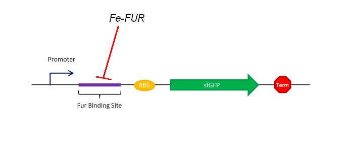
Naturally, when there is a large amount of iron in the environment, 2 iron ions complex with 2 FUR proteins and bind to the FUR Binding Site (FBS). This interaction regulate negativelly the genes downstream.
As shown on the Figure 1, our sensing system relies on a FBS. In order to easily model the sensing delay and analyse its results, the first construction is composed of a GFP placed right after the FBS.
Goals
Our goal in this part of the model is to create a generic FBS-related sensing model so that:
- We can determine the iron-sensing delay of our bacteria
- The model can be reused by other projects that include a FBS sensor
Materials and methods
From Iron to FBS:
The iron-FUR complex is simply formed that way:

We reduced this equation to:

Which is not annoying, since we just have to divide our [FeFur] by two to get the real complex concentration.
We can easily write down both the formation (v) and the dissociation (v') speeds:

We chose to model the iron input in the bacteria using a linear function of the external iron concentration Ferext, the factor p being the cell-wall permeability for iron.
The FUR on the other hand is produced by the bacteria. Its evolution can also be considered as linear, using a mean production rate of Fur0.


In this model, we only track the free Fe-FUR complex and not those attached to a FUR Binding Site. FBS is the number of inhibited Fur Binding Sites.

GFP expression:
To simulate the inhibition phenomenon, we chose to use our Logistic function under its differential form. Since it is the Fe-FUR that represses it, the LacI can be expressed as a logistic fuction of the Fe-FUR:

Ki1 is a non-dimensional parameter that repesents the inhibition power, and Kf is the fixation rate of the Fe-FUR on the FBS. Finally, Npla1 is the number of pasmids containing the GFP.
GFP Production:
The [mRNA] and [GFP] equations are alike. The prodction rates are Kr for the mRNA and Kp for the GFP. Since FBS represents the number of inhibited Fur Binding Sites, we have to substract it from Npla1.
Both variables also have a negative degadation term:

Tuning the model
The only parameter we couldn't find in the litterature is Ki1. Nevertheless, thanks to our construction and the experimental results we obtained with a plate reader, we can tune this parameter to obtain a realistic sensing model!

The Figure 2 is a set of experimental results showing the sensing efficiency for different iron concentrations. We can notice a substantial behaviour change between 10-4M and 10-5M of iron : the activity of our bacteria leaps at 10-5M.
Therefore, we ran simulations with different Ki1 values to try to determine the most fitting Ki1.

The Figure 3 shows that our model can lead to 3 different leaps, depending on the Ki1 value. The leap we are interested in is the 10-4M 10-5M leap.
We thus zoomed in, and performed the simulations with a more adapted range of Ki1.

The Figure 4 shows a more precise graph. It is with those simulation values that we calculated the most realistic Ki1, by maximizing the leap it creates. We also figured that the best fitting case requires the GFP reaching a plateau right after 10-5M of iron.
Finally, we set Ki1 at 6,3.10-5.
Results
The following results were computed using those parameters:
| Name | Value | Unit | Description |
|---|---|---|---|
| p | 0.1 | min^-1 | Permeability of cell wall |
| KFeFUR | 0.01 | M-1.s-1 | Formation constant of FeFur complex |
| Dff | 0.001 | min-1 | FeFUR degradation rate |
| Kp | 0.5 | min-1 | translation rate |
| NA | 6.02*1020 | mol-1 | Avogadro's constant |
| V | 6.5*10-16 | m3 | Volume of a bacterium |
| DmRNA | 0.001 | min-1 | mRNA degradation rate |
| Kf | 10-4 | min-1 | fixation rate of FeFUR |
| Fur0 | 0.01 | mM.min-1 | Fur Production rate |
| Ki1 | 6,3.10-5 | - | Sensor efficiency |

As shown in the Figure 5, there is a significant change in GFP production after 1000 seconds between the curve at 10-4M of iron and the one at 10-5M. The bacteria can thus sense low concentrations of iron.
Conclusion
The first construction of our team is fully modeled : we made a generic iron sensing model (with the FBS system).
Thanks to the experimental results we obtained with a plate reader, we were able to tune an unknown parameter to obtain a more realistic model.
This sensing model allowed us to continue the Enterobactin production model, the next step being the Inverter model.
Models and scripts
This model was made using the Python language. You can download the python script here.