 "
"
Team:Freiburg/Project/modeling
From 2013.igem.org


Modeling our dCAS
Introduction
We used a kinetc approach to model and characterize our system. It is based on various ordinary differential equations (ODE) which describe the behaviour of our network. Due to the limited measurement possibilities and the unwritten law, that you should at least measure half of the number of components of your network we started by using a small network with a limited amount of different components.
The Networks
1. dCAS-VP16
Our network includes four different components dCas9-VP16, a RNA complex (tracr/cr RNA), a RNA-dCas9-VP16 complex and the secreted alkaline phosphatase (SEAP). The RNA-complex is bound to dCas9-VP16 and the resulting complex binds the DNA, which leads to the production of SEAP.
 |
| Figure 1: Transcriptional Activation via dCas9-VP16: The dCas9-VP16 fusion protein is guided to the desired DNA sequence by a co-expressed crRNA and tracrRNA. The binding of the gene recognition complex leads to an expression of SEAP. |
Setting up the ODE
According to the graphical reaction network the ODE can be set up.
dCas9 is constitutively expressed by the CAG promoter and degraded proportionately to the current concentration. It is used to build the DNA recognition complex and is produced during complex decay.

The RNA-complex is built linearly. The production constant can be regarded as equivalent to the production constant of the lower expressed RNA (either crRNA or tracrRNA), since their expression limits the complex building. It is assumed that the RNA is degraded after DNA recognition complex decay and therefore the complex decay does not lead to an increase in the amount of RNA.

The DNA recognition complex is built when dCas9 and RNA meet and is degraded proportionately to the current DNA recognition complex concentration.

There is a leaky SEAP production and one that depends on the current concentration of the dCas9/RNA complex. This dependency is assumed to follow the Monod-kinetic. Because of the long half-life period (T2 > 500 h) of SEAP we can neglect the SEAP decay [2, 3].

| The parameters are: | |
|---|---|
| k1: linear production rate of Cas9 k2: Cas9 degradation rate k3: tracr/crRNA production rate k4: tracr/crRNA degradation rate k5: gene recognition complex building rate |
k6: cr/trRNA /Cas9 degradation rate k7: SEAPs leaky production rate k8: Complex dependent SEAP production rate k9: Cas9-VP16 specific constant |
2. dCAS-KRAB
The dCas-KRAB sytem was modeled as a three component system. tetR as activator of gene production, dCas-KRAB as repressor and SEAP as final reporter protein.
 |
| Figure 2: Transcriptional respression via dCAS-KRAB: The dCAS-KRAB fusion protein binds to the desired target sequence at a different locus than the tetR. tetR in turn binds to tetO and is assumed to repress SEAP production. |
Setting up the ODE
According to the graphical reaction network the ODE can be set up.
dCas9 is constitutively expressed by the CAG promoter and degraded proportionately to the current concentration, similar to the activation model. It binds to the DNA and is released afterwards. Since the amount of transfected dCas9-plasmid is four times higher than that of TetR-VP16 the basal expression rate is equally assumed to be four times higher than that of TetR.

tetR is assumed to have a similiar kinetic as dCas9.

There is a leaky SEAP production and one that depends on the current concentration of dCas9 and tetR. This dependency is assumed to follow an allosteric inhibition process. Similar to the activation process the SEAP decay can be neglected because of the long half-life period (T2 > 500 h) of SEAP [2, 3].

| The parameters are: | |
|---|---|
| k1: linear production rate of Cas9 k2: Cas9 degradation rate k3: tetR production rate k4: tetR degradation rate |
k5: SEAPs leaky production rate k6: Cas9/tetR specific production rate k7: Cas9-KRAB specific constant k8: tetR specific constant |
Determining the parameters
By setting up the ODE a (n+1)-dimensional hypothesis space (n is the number of
parameters) is generated. Determining the right parameter combination means finding a point in the space which fits the data best.
To find these parameters we used the maximum likelihood approach. The maximum likelihood hypothesis is the procedure which has the highest probability to
generate the measured data. It was shown, using the maximum likelihood approach and assuming gaussion noise to the data (an assumption that holds in our case) leads to a least-square error minimization problem [3].
A minimization problem is an optimization problem. One searches for parameters (p0) for which the assumption holds, that the value of the function (f) at the point of the parameters is smaller than all other values (f(p0)<=f(p)). In three dimensions the function can be regarded as a landscape and minimization as finding the deepest valley. Depending on the method one uses different problems arise. The most common problem is finding an only local minimum instead of the global one (Fig. 3).
 |
| Figure 3: Example of a minimization problem A 3D landscape is shown. Depending on the start position (the initial parameters), the minimum which is found can either be a local minimum or the global one. |
To avoid this issue and to make sure a global minimum was found we started our minimization procedure using different start values for our parameters. To sample these parameters we used the latin hypercube sampling on a logarithmic scale (Fig. 4).
 |
Figure 4: Illustration of the latin hypercube sampling in a two dimensional parameter space. The number of initial parameter vectors is 5. Therefore the parameter space is divided in 25 subspaces. One possible parameter combination is shown here. |
The number of different initial parameter settings is set to N and thus the parameter space is divided in N*N subspaces. For the initial parameter the values are chosen in a way that there is only one parameter in each row and column.
The resulting errors were plotted in an increasing order to be sure the global minimum could be found.
Data generation
Fusion proteins with effectors (dCas9-VP16, dCas9-KRAB) were quantified, as well as SEAP reporter protein (secreted alkaline phosphatase).
1. dCas9-Effector Quantification
dCas9-VP16 and dCas9-KRAB were quantified by using Western Blots.
 |
| Figure 5: Western Blot quantification of protein concentrations. |
2. SEAP Reporter Quantification
SEAP reporter protein was quantified by using a SEAP assay.
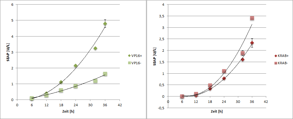 |
| Figure 6: SEAP reporter protein quantification by using the SEAP assay. |
For more detailed information refer to our modeling notebook.
Fitting Procedure and Results
1. dCas9-VP16
Assuming the given ODE and using the fminsearch-function of matlab for various initial parameter vectors the fitting process resulted in one optimal parameter composition. Our measurement time started with a transfection. The first data were obtained after 6 h. As the initial concentrations were unknown all 14 parameters (including the initial concentrations) were assumed to obtain changing values during the fit. This procedure results in unlikely high initial concentrations. Although the transfection end point could not clearly be defined only a small amount of the components should be present within the cells after transfection . A second process in which the initial concentrations were assumed to be zero followed the first one. The change between fixed and variable parameters was easy to perform, because of an additional vector (qfit). This vector contained different boolean values depending on whether the parameter was fixed (false) or flexible (true) during the fitting process. Moreover another parameter was required for adjusting the absolute values of the duplicates. The results of this second process are shown in table 1.
The model reflects the general construction of the network (Fig. 5). As assumed dCas9 converges asymptotically to a steady state and an exponential increase in the SEAP concentration can be observed. Both processes are reflected in the data.
The model also shows a potential behavior of the non measured components, the free tracr/crRNA-complex and the gene recognition complex. The tracr/crRNA-complex reaches its steady state quickly. However there is no possibility to distinguish between the two different RNAs. There might be some differences in their expressions, especially because of the different promoters (crRNA expressed under U6-promoter; tracrRNA expressed under h1-promoter), however, the model does not show them.
The free gene recognition complex has not reached its steady state yet due to the small degradation rate.
 |
| Figure 7: Modeling Result: This figure shows the comparison of the experimental results (purple square) to the model prediction values (cyan cross) for SEAP and dCas9, as well as the model prediction for non measured components. |
Since the fminsearch algorithm is not proved to converge to a minimum [1], different points within the parameter space were chosen to ensure a high probability for finding the global minimum (Fig. 8).
 |
| Figure 8: Different error values plotted in increasing order. |
| parameter | value |
|---|---|
| linear production rate of dCas9 | 8.78E+02 [M/h] |
| dCas9 degradation rate | 0.54 [1/h] |
| tracr/crRNA production rate | 0.73 |
| tracr/crRNA degradation rate | 1.21E+08 |
| Gene recognition complex building rate | 1.61 [1/M] |
| cr/trRNA /dCas9 degradation rate | 8.59E-26 |
| SEAPs leaky production rate | 4.05E-05 [M/h] |
| Complex dependent SEAP production rate | 1.86E+08 [M/h] |
| Cas9-VP16 specific constant | 1.06 |
| initial concentration: dCas9 | 0.00 [M] |
| initial concentration: tracr/crRNA -Komplex | 0.00 |
| initial concentration: gene recognition complex | 0.00 |
| initial concentration: SEAP | 2.73E-09 [M] |
| least square error | 159.3423 |
Using the Model
The parameters of our model were identified by using MATLAB and a least square error minimization procedure. Afterwards the model, written in SBML by using COPASI, was used to test how the amounts of reporter protein can be increased by changing other parameters. As assumed the reporter protein level depends on the concentration of RNA and dCas9-VP16. If one paramter is increased, reporter level rises.
We decided to try to increase the dCas9-VP16 expression rate, because there are no possibilites to increase the RNA amount. The promoters coding for the RNAs are classified as strong and it's not possible to shorten the sequences. dCas9 in contrast is a large protein - over 160 kDa - and has various functions. Basically we need only the helicase and DNA binding domain. Therefore it should be possible to remove other domains by truncating the protein and so reducing the protein's size. When the protein is smaller, we expect that the dCas9 expression will increase. This will lead - according to the model - to a higher output of the system.
There are several other possibilities of increasing the expression rate practically:
One is to change the promoter, another one means transfecting more plasmid DNA and - as already mentioned - there is the possibility to truncate the protein itself. Although a change of the promoter seems to be the most simple method, we couldn't perform this, because we already used the strong CAG promoter. By transfecting more plasmid DNA the toxic effects on the cells will increase.
This is why we decided to truncate the dCas9-VP16. We assumed that by reduction of size of dCas9-VP16 with the same amount of cellular resources more protein can be built. A positive side effect might therefore also be that the off target effect on the regular protein translation goes down, as well.
To read more about the truncation click here.
 |
| Figure 9: Parameter Scan The theoretical behaviour of the dCas9-VP16 concentration and the SEAP concentration by various dCas9-VP16 production rates. |
2. dCas9-KRAB
The same procedure was performed to find the parameters for dCas9-KRAB. All parameters were set to changing values and the initial concentrations to zero. Fitting applied to initial concentrations of zero led to a lower least square error. As assumed before the dCas9-KRAB reaches its steady state within the measured time period, approximately at the same time point as Cas9-VP16. However the expected stop of the increase in SEAP concentration could not be observed. The effect of repression is unobservable due to the high ratio of tetR to dCas9.
 |
| Figure 10: Modeling Result: Experimental results (purple square) are shown in comparison to the model prediction values (cyan cross) for SEAP and dCas9, as well as the model prediction for the non measured component tetR. |
This time we also fitted the different error values (Fig.11).
 |
| Figure 11: Different error values plotted in increasing order. |
| parameter | value |
|---|---|
| linear dCas9 production rate | 7.04E-04 [M/h] |
| dCas9 degradation rate | 1.55E+02 [1/h] |
| tetR production rate | 5.59E+09 |
| tetrR degradation rate | 1.29E-04 |
| SEAPs leaky production rate | 2.70E-15 [M] |
| Cas9/tetR specific production rate | 0.18 [M] |
| Cas9-KRAB specific constant | 1.27E+00 [1/M] |
| tetR specific constant | 4.30E+13 |
| initial concentration: dCas9 | 0.00 [M] |
| initial concentration: tetR | 0.00 |
| initial concentration: SEAP | 8.90E-19 [M] |
| least square error | 119.6221 |
The Code Files
References: