"
"
Team:Evry/LogisticFunctions
From 2013.igem.org
| Line 30: | Line 30: | ||
<p>The solution of this Cauchy problem is as below:<br/> | <p>The solution of this Cauchy problem is as below:<br/> | ||
| - | + | <img src="https://static.igem.org/mediawiki/2013/3/3d/Solution_cauchy.jpg"/> | |
| - | + | ||
</p> | </p> | ||
Revision as of 15:42, 29 September 2013


Logistic functions :
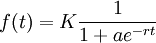
When we started to model biological behaviors, we realised very soon that we were going to need a function that simulates a non-exponential evolution, that would include a simple speed control and a maximum value. A smooth step function.
Such functions, named logistic functions were introduced around 1840 by M. Verhulst.
These functions looked perfect, but we needed more control : we needed to set a starting value and a precision.
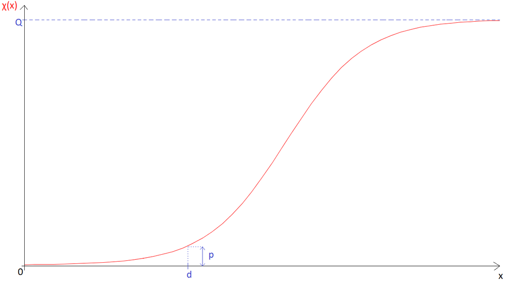
Parameters:
- Q : Magnitude.
The limit of g as x approaches infinity is Q. - d : Threshold.
The value of x from which we consider the start of the phenomenon. - p : Precision.
g(d)=Q*p Since the function never reaches 0 nor Q, we have to set an approximation for 0 or Q. - k : Efficiency.
This parameter influences the length of the phenomenon.
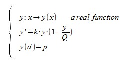
Differential form:
Let the following be a Cauchy problem:
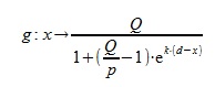
The solution of this Cauchy problem is as below:
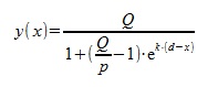
Here is our logistic function. Yet, differential equations are not always time-related.
Let x be a temporal function, and y be a x-related logistic function. In order to integrate y into a temporal ODE, we need to write it differently:
dy/dx = by(x(t))(1 – y(x(t))/K)
<=>( dy/dt)/(dx/dt) = by(x(t))(1 – y(x(t))/K)
And so:
dy/dt = dx/dt * by(x(t))(1 – y(x(t))/K)
If t → x(t) is a continuous real function, then:
y(x(t)) = y(t)
Finally,
dy/dt = dx/dt * by(1 – y/K)
References: