Team:Evry/Modeltr1
From 2013.igem.org
Disease model
Introduction
In the very beginning of the project, we focused on iron absorption by the duodenum. We first had to model the behaviour of the duodenum regarding iron absorption to determine if a flush treatment strategy was viable.
Observations
We know that 60% of iron is absorbed in the duodenum and 40% in the jejunum. The duodenum is located in the upper intestines, right after the stomach, and is usually 300mm long.
A healthy person absorbs about 10% (1-2mg a day) of the daily iron uptake, while a hemochromatosic patient's absorption varies between 50% and 100% of the daily iron uptake[1].
Iron absorption is normally regulated by the liver through hepcidin production (depicted in Figure 1). This means that after a certain delay, iron absorption eventually reaches a stationary phase.
Goals
We wanted to build a generic duodenal iron absorption model so that:
- We can have a realistic base for the Final flush treatment model
- The model can can be reused in the future for any similar model of absorption.
Assumptions
- Our bacteria doesn't settle in the duodenum
- No regulation of the patient's iron absorption
- Constant iron flow in the duodenum lumen
- Homogeneous fluid
- The bacterial quantity is constant
- The bacterial natural absorption is insignificant compared to the chelation
- The patient ingests 20mg of iron per day (Guideline Daily Amounts)
Materials and methods
This model simulates the digestion process of one meal from the duodenum's point of view.
The duodenum is considered as a cylinder in which a homogeneous fluid flows. The model is divided into three steps: the filling of duodenum, the steady state flowing step and the emptying.
This model has two variables : the iron dissolved in the duodenum lumen (S) and the absorbed iron (A).
We considered the chyme arrives in the duodenum at a constant rate. S has a linear component Sp which represents the pulses. The also are an emptying component and an absorption component.
We assumed a linear absorption and a negative feedback regulation for A.
Finally:

|
|
Parameters tuning :
As the iron absorption process greatly differs from an individual to an other, α and σ cannot be related with anything in the litterature. We thus had to tune those parameters.
First of all, we know that a hemochromatosic patient absorbs at least 50% of the iron he ingests. Thus, we tuned α to fit this information while assessing σ = 0 (Hemochromatosis : no regulation in iron absorbtion).
Then, since we know that a healthy person absorbs 10% of the ingested iron, we were able to tune σ.
Results
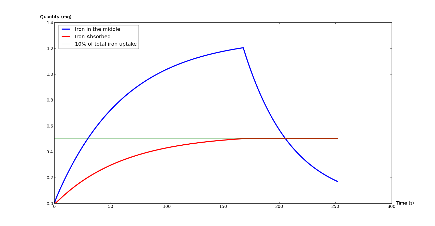
These curves represent the total absorbed iron (in red) and the instant iron quantity in the duodenum lumen (blue).
The green line is a landmark: it represents the iron absorption of a healthy person during an average meal.
The Figure 2 represents what would normally happen during an average meal. It will be a sample graph for our model.
The Figure 3 was generated with the same equations as the Figure 2, but where σ = 0, which means that there is no regulation of iron absorption.
Parameter values
| Name | Value | Unit | Description | Reference |
| Sp | 0.03 | mol.s-1 | Iron pulse | [1][2] |
| v | 7*10-3 | m.s-1 | Chyme's flow average speed | [2] |
| L | 0.3 | m | Duodenum length | [3] |
| α | 0.3 | s-1 | Duodenum absorption rate | tuned |
| σ | 0.72 | s-1 | Regulation coefficient | tuned |
Sensitivity Analysis
As two parameters cannot be tuned: α and σ, we had to study the stability of the model with respect to the change in these parameters.Model response in function of α
We start by varying α and keeping σ to its tuned value. This gives the results presented in Figure 4 below.The dynamic of the model is not changed α < 1 but, as α gets bigger, the absorbed iron increase greatly, crossing the green (maximal absorption for healthy patient) for α < 10.
Model response in function of σ
We do the same simulations with different values for the σ parameter, keeping the α to its tuned value. The result of these simulations is presented in Figure 5.
As expected with the equation, the σ parameter shows a sigmoid decreasing shape affecting a lot the iron absorption.
Model response in function of α and σ
As the model possesses only two free parameter, it is possible to do the joint analysis of the two parameters. This analysis is shown in FigureConclusion
This model provides rational results regarding the iron absorption phenomenon. Therefore, we will be able use it as a base for the next simulations.
The next step is to include our bacterial flow in this model, which will result in the Final flush treatment model.
Models and scripts
This model was made using the Python language. You can download the python script here.
 "
"


