 "
"
Team:UANL Mty-Mexico/Modeling
From 2013.igem.org
Mathematical models that represent the dynamic behavior of biological systems are a quite prolific field of work and are pillar for Systems Biology. A number of deterministic and stochastic formalisms have been developed at different abstraction levels that range from the molecular to the population levels.
In principle, a model that is simple but that is good enough to describe and make predictions, with a degree of certainty, about the phenomenon under scrutiny, would be desirable.
Deterministic mathematical models that describe the behavior of genetic circuits and the interactions of the proteins they encode are usually built upon mass action kinetics theory.
Aside from the common objection that they are not suitable to describe systems that show a low number of particles, we believe that a deterministc model at a molecular level of these kind of systems and the degree of certainty with which they can be used for inter-system comparison or usage, do not outweigh the costs of the experimental determination of parameters.
Here we propose a model for the description and comparison of the behavior of the effect of RNA thermometers or RNATs on the expression of a reporter protein. The model is tested with relative fluorescence units data, which are not hard to obtain, and the model and its parameters should allow for inter-system comparisons, i.e., to compare the temperature-dependent gene regulation features of different RNATs; an extension that works with protein concentration units is also proposed, along with a potential application in metabolic engineering, and waits for experimental validation.
We present a model for the relation between time, temperature and the change in fluorescence (measured in Relative Fluorescent Units or RFUs) of an E. coli culture that harbors a genetic construction where a fluorescent protein is under control of a RNAT.
Giving the organization of our circuit we will expect the temperature to be the main factor involved in regulation of the fluorescence, where first we will have an off state, followed by an optimal fluorescence and then ending in an off state again, the time will have almost the same effect as it does in any other giving biological phenomena involving gene expression.
Using this model we intend to have the same conditions at the time of the fluorescence measurements so we expect to not have conditions such regarding the incubation (Expect for the temperature) to have a significant effect in the fluorescence.
Although the same conditions will be used the strain used to test the circuit could have and influential effect giving the metabolic and genetic conditions of living.
We took as reference for the RFUs the amount of fluorescence emitted by an E. coli K12 culture transformed with a constitutively expressed part BBa_E1010 (for RFP expression) or BBa_E0040 (for GFP expression) per unit of Optical Density at 600 nm light (OD600) after 8hr of growth at 37°C in LB medium.
In this way the amount of fluorescence emitted by our culture was calculated as follows:
\begin{equation} \large F_{R} = \frac{F_{sample}}{F_{standard}} \end{equation}where Fsample is the OD600-normalized fluorescence emited by a sample, while Fstandard is the OD600-normalized fluorescence measurement for the corresponding standard culture (again, BBa_E1010 for RFP and BBa_E0040 for GFP).
During our experiments to measure the fluorescence produced in the cell cultures, we had the same unchanging global conditions (temperature, initial conditions, and medium used to grow cells).
For each measured in a giving temperature, the system was left until a point in which we were sure the O.D of the cell culture and the production of the protein were in equilibrium, steady, and uniform, before the cells population started to decrease.
After a few test between different hours it was found that, for our cell cultures,it was around 15 hours and 20 hours so our measurements were made at 17 hours from the start of the growth. Thus, we can say these fluorescence measurements were Steady State measurements, in which the system was in equilibrium.
Our measurements were made in LB medium at 25, 30, 37 and 42°C, for each one of our constructions that are part of the whole circuit.
Steady State: Referrers to the condition or conditions of a physical system or process that does not endure a change over time, or in which any given change is continually balanced by another, such as the stable condition of a system in equilibrium.
Parameter estimation: is the process or method used when trying to calculate mathematical model parameters based on experimental data sets through numerical methods. These data sets can be the result of steady states of independent events or time course experiments. Although there are numerical methods to do this, more complex algorithms with great accuracy are already incorporated in most of the new mathematical software, such as COPASI and MATLAB.
More deeply, Estimation Theory is a branch of Statistics and Signal processing that deals with estimating the values of parameters based on measured/empirical data that has a random component (deviation or unknown tendency). The parameters describe an underlying physical setting in such a way that their value affects the distribution of the measured data. An estimator attempts to approximate the unknown parameters using the measurements, trying to adjust these parameters to fit the model to the experimental data.
The best numerical method for the estimation of parameters through COPASI resulted to be the Evolutionary Programming. Another way to do this parameter estimation, is performing a Function Fit of its analytical solution, which is shown in the Appendix, at the end of this page.
Let's consider the change of the relative fluorescence of a sample with respect to time. This change can be described by the following differential equation:
\begin{equation} \frac{dF_{R}}{dt} = \alpha - \delta F_{R} \end{equation}Here, \(\alpha\) is the production rate (in RFUs per unit time or \(RFU min^{-1}\)) and \(\delta\) is the degradation rate (in reciprocal unit time units or \(min^{-1}\)).
This is the familiar production and degradation model whose steady state can be expressed as follows:
\begin{equation} \ F_{Rst} = \frac{\alpha}{\delta} \end{equation}Now, we assume that after growting for 8 hours at a given temperature, a culture would have reached the steady state OD600-normalized fluorescence expression. Taking this assumption into account, we can plot the value of \(F_{Rst}\) after growth at different temperatures and find a function that we will call \(f(T)\). Note that we use capital \(T\) to distinguish temperature from time, for which we use lower case \(t\).
If we merge this assumption to equation 3, we have:
\begin{equation} \ F_{Rst} = f(T) \end{equation}In Shah and Gilchrist, (2010), it was found that the probability of openness of a ribosome binding site (RBS) of an mRNA with respect to temperature, fits well into a logistic equation. However, the authors did not find significant differences in the behaviour of known RNATs and non-RNAT elements and admit that RBS openness cannot be assumed to be directly correlated to translational activity. Therefore, their RBS-melting probability equation would not be recommendable to be used directly in gene expression models for RNATs.
However, because other factors may be involved in RNAT-mediated gene regulation, such as the effect of ribosome binding and other structural features, we can still assume there is an unknown function that takes into account these effects. We initially tried with a logistic model, but our data seems to be more in concordance with a Gaussian distribution.
The most accessible measure of fluorescence emission that we can get to find a relation with temperature, is the steady state fluorescence emission of our system at a given temperature, which we already called \(F_{Rst}\).
Our dynamic model is reduced in complexity when \(F_{st}\) is known -which is the case when we let grow the cells until they reach a stable fluorescence measurement-. It can be used to construct a model in COPASI [Hoops, S., et al., (2006)] and experimental data can be fitted to the equation and empiric estimations for \(\delta\) can be obtained. This estimations can be used to compare the behavior of different RNATs, whenever they are tested under the same standard conditions that we have described through out the text (i.e., using the same standards to normalize OD600 data and growing their culture in the same conditions).
However, due to time restrictions, we weren't able to take time series measurements of cultures growing at different temperatures. We simulated the behavior of our system using different values for the \(\delta\) parameter and the parameters obtained for the \(f(T)\) function.
We are also aware that as temperature increases, the overall degradation rate of proteins also does. In consequence, we expect to see a rise in the degradation rate in our dynamic model as temperature increases. If we plot the value of \(\delta\) obtained at different temperatures, we will end with a function \(\delta(T)\) that shows an unknown form:
\begin{equation} \frac{dF_{R}}{dt} = \delta(T) \large{(}f(T) - F_{R}\large{)} \end{equation}Nevertheless, this is a consideration that we'll leave for further analysis and for now, we'll assume that \(\delta)\ does not change significantly in the chosen temperature range (25 - 42°C).
In mathematics, a Gaussian Function (named after Carl Friedrich Gauss) is a function of the form:
\begin{equation} \ f(x) = a e^{\frac{-(x-b)^{2}}{2c^{2}}} \end{equation}for some real constants a > 0, b>0, c> 0, and Euler's number).
For which MATLAB uses the following custom equation when fitting data to a Gaussian Function:
\begin{equation} \ f(x)= a e^{\frac{-(x-b)^{2}}{c^{2}}} \end{equation}Where 2c is considered as c for simplicity the normalization of x, b is the mean (average) and c the standard deviation.
For us, we are using this function as a model for the dependency of the Relative Fluorescence of each construction. Its equation would be the following:
\begin{equation} \ F_{Rst}(T)= a e^{\frac{-(T-b)^{2}}{c^{2}}} \end{equation}The parameter a is related to the amplitude of the function. This is important for the model, because higher amplitudes will provide a better signal, and will not be lost among noise background.
The parameter b is related to the horizontal shift. A better interpretation of it is the value of x where the function has its higher value. For us this is the optimal temperature of the RNAT.
The parameter c is related to the width of the bell. This is important for the application of this model for RNAT, because smaller width will mean a more clear and defined signal.
Some important biological phenomena are described in this function giving a bell curve for example the length of a specific bird beak, following this equation the majority of the population of a the specie will show a range of values that culminates in a mean value being generated. The central peak of the bell curve will show the modal average, and the highest frequency of results will be shown in this space.
Another example will be the activity of an enzyme at a certain temperature likewise to this model this proteins have a temperature rage for optimal structure and functionality, this will be shown in a bell curve where we will have a relation between the temperature and function of the enzyme, we will observe the maximum function of the enzyme in the central peak of the bell curve giving that there will be function in nearby temperatures but it will have a gradual decrease until it stops functioning either at a higher or a lower temperature.
It is a basic and fairly accurate model of how different characteristics, or traits, are carried through a sample of organisms, and how certain conditions provide an optimal function or higher survival rate among a biological system.
We are choosing the Gaussian Function, because of the relevance that its parameters have for our model. Defining these parameters will provide us a way to quantify the strength (a), optimal value (b), and definition or clearness (c) of our RNAT activity.
We analyzed the data obtained from the 4 clones derived from the transformation with Part:BBa_K110006 (see wetlab section), called M1, M2, M11 and M12. The results for the Gaussian Function Fitting are shown in the following figures (all the following figures were done within Matlab, as well as the fitting of the functions):
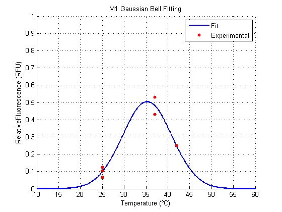
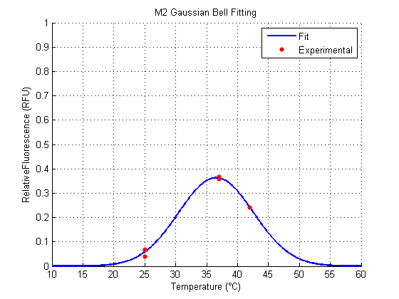
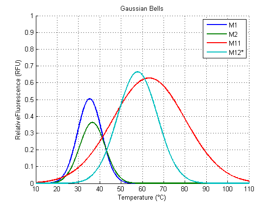
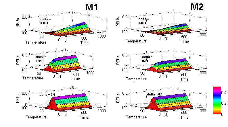
Both M1 and M2 have a similar behavior (figures 1, 2). They show an optimal Relative Fluorescence around 37°C. M2 seems to have a better fit to the data than M1, while M1 (around 0.5 RFU) has greater amplitude than M2 (around 0.4 RFU).
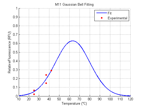
The results for M11 and M12 have a fit that doesn’t follow a biological interpretation (figures 3,4), because they seem to have (according to a Gaussian Function Fit) an optimal temperature around values higher than the viable temperature for the microorganism we are working with. This is because they show a slower (or shifted) increase of Relative Fluorescence in relation to the others.
However, the gaussian function of M1 and M2 could be potentially predictive for non-verified temperatures and even distinct RNATs.
In the following section, we show the result for the parameters.
| Clone | a | amin/max | b | bmin/max | c | cmin/max |
|---|---|---|---|---|---|---|
| M1 | 0.5042 | 0.3594/0.6490 | 35.2700 | 32.9600/37.5800 | 8.0180 | 5.6810/10.3500 |
| M2 | 0.3630 | 0.3309/0.3950 | 36.5300 | 35.5300/37.5200 | 8.5250 | 7.5210/9.5300 |
| M11 | 0.6283 | -5.4200/6.6770 | 63.1300 | -141.3000/267.6000 | 24.0900 | -63.4000/111.6000 |
| M12plus | 0.6646 | -57.64/58.9700 | 57.7300 | -789.0000/904.4000 | 13.1800 | -291.1000/317.4000 |
| M12 | 0.1914 | -inf/+inf | 41.49 | -inf/+inf | 1.225 | -inf/+inf |
| RFP | 1.0000 | 0.8088/1.1910 | 38.2300 | 34.5700/41.8900 | 10.3700 | 6.5230/14.2100 |
For the parameter a, which represent the strength of the signal, M1 is the better one among the clones, excluding the result of M11 and M12, because they show their respective peaks far away from the accepted range of temperatures approximately around 20°C and 50°C.
For the parameter b, which represent the optimal temperature for the RNAT (the ON state), M1 and M2 behave more likely to what we expected. The same happens for the control RFP. All these are around 37°C. For M11 and M12 (for its both cases), optimal temperatures are away from what we expected, and what would work for between the accepted temperatures.
For the parameter c, which represents the width (clearness or definition) of the signal, the smallest (best) clone was M1. M12 is not considered because it has a very poor amplitude and a shifted optimal temperature.
| Clone | SSE | R2 | AdjustedR2 | RMSE |
|---|---|---|---|---|
| M1 | 0.0066 | 0.9637 | 0.9396 | 0.0471 |
| M2 | 0.0005 | 0.9953 | 0.9922 | 0.0134 |
| M11 | 0.0055 | 0.9041 | 0.9041 | 0.0430 |
| M12plus | 0.0001 | 0.9956 | 0.9867 | 0.0083 |
| M12 | 0.0092 | 0.7161 | 0.5268 | 0.0553 |
| RFP | 0.0266 | 0.9710 | 0.9516 | 0.0941 |
The last table shows the confidence parameters (SSE, R2, Adjusted R2 and RMSE) that Matlab provides for each fit. For the first and last column, smaller values mean less error or deviation of the model to the data. For the other two parameters, the closer the values get to 1, it means it has a better fit.
M12 has a particular behaviour compared to the other clones, which is of great interest but need further and deeper analysis. For the previous analysis, M12 represent a restricted range of our data set for which we are more confident of the results.
For more insights around this special case, refer to Results, in the section Wetlab.
- Shah P and Gilchrist MA (2010) Is Thermosensing Property of RNA Thermometers Unique? PLoS ONE, 5(7):e11308.doi:10.1371/journal.pone.0011308.
- Von Fircks HA and Verwijst T (1993) Plant Viability as a Function of Temperature Stress (The Richards Function Applied to Data from Freezing Tests of Growing Shoots) Plant Physio, 103(1):125–130.
- Hoops S, Sahle S, Gauges R, Lee C, Pahle J, Simus N, Singhal M, Xu L, Mendes P and Kummer U (2010) COPASI–a COmplex PAthway SImulator Bioinformatics, 22(24):3067-3074,2006,http://dx.doi.org/10.1093/bioinformatics/btl485
- COPASI Documentation 2.Steady State calculation (May 16, 2013). Retrieved from http://www.copasi.org/tiki-integrator.php?repID=9&file=ch07s02.html
- Chen T, He HL and Church GM. (1999) Modeling gene expression with differential equations Pacic Symposium of Biocomputing29-40
- Gaussian function (Consulted on September 27, 2013) Retrieved from http://uqu.edu.sa/files2/tiny_mce/plugins/filemanager/files/4282164/Gaussian%20function.pdf
Here we are going to show how we solved the differential equation 5.
First we choose to solve it through separation of variables. Thus we move every term with \(F_{R}\) to the left side of the equation, and everything else in the right side:
Then we proceed to integrate but sides of the equation:
The left integral has the solution of a natural logarithm, while the right side, as \delta is constant for constant temperature, has a simple solution:
Then we apply the exponential function in both sides of the equation:
Rearranging the equation, through laws of exponents, we can change the right side like this:
The exponential of \(C\) can be treated as another constant, that we will call \(K\):
There by:
\begin{equation} \ F_{R}= F_{Rst} + K \ e^{- \delta {t}} \end{equation}
