Team:ETH Zurich/Modeling/Analytical Approximations
From 2013.igem.org
| Line 34: | Line 34: | ||
| - | + | <h1> Solution at the steady state </h1> | |
| - | < | + | The steady state solution is described by the differential equation |
| - | + | ||
\begin{align} | \begin{align} | ||
| - | + | 0 & = & C_{agar} \cdot D_{AHL} \left(\frac{1}{r} \frac{\partial [AHL](r, t)}{\partial r} + \frac{\partial^2 [AHL](r, t)}{\partial r^2}\right) - d_{AHL,e} \cdot [AHL] (r, t) | |
\end{align} | \end{align} | ||
| - | |||
| - | |||
| - | |||
| - | |||
| - | |||
\begin{align} | \begin{align} | ||
Revision as of 01:00, 29 October 2013
Contents |
Steady State AHL Gradient Approximation
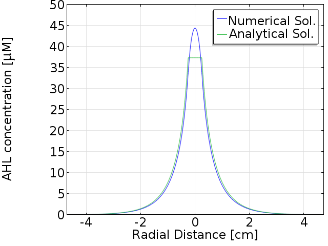
In the reaction-diffusion model we have formalized the gradient establishment and we solved the resulting partial differential equation numerically. Now, the aim is to derive a suitable analytical approximation for a single mine colony.
Kolmogorov-Petrovsky-Piskounov Equation
We consider the Kolmogorov-Petrovsky-Piskounov equation, i.e., the reaction–diffusion equation concerning the concentration of a single molecule. In our case we consider two spatial dimensions, and the equation for AHL then has the following general structure:
\begin{align} \frac{\partial AHL(r,\theta,t)}{\partial t} = Diff(AHL(r,\theta,t),x) + R(AHL(r,\theta,t)) \end{align}
We were interested in the AHL gradient that can be established by a single colony (located at $r = 0$ with radius $R = 2.5mm$) on an agar plate, ending up with a less general form of the reaction-diffusion model for AHL. The dependency on the angle $\theta$ can be disregarded the gradient established in two dimensions is radially symmetric. The polar coordinate Laplace operator for such a problem is
\begin{align} \nabla^{2} f = \frac{1}{r} \frac{\partial f}{\partial r} + \frac{\partial^2 f}{\partial r^2} \end{align}
The reaction-diffusion equation (Gordon et al., 2013) then reads
\begin{align} \frac{\partial [AHL](r, t)}{\partial t} & = & C_{agar} \cdot D_{AHL} \nabla^{2} [AHL](r, t) - d_{AHL,e} \cdot [AHL](r, t) \\ & = & \frac{1}{r} \frac{\partial [AHL](r, t)}{\partial r} + \frac{\partial^2 [AHL](r, t)}{\partial r^2} - d_{AHL,e} \cdot [AHL] (r, t) \end{align}
with boundary conditions
\begin{align} - D \frac{\partial [AHL]}{\partial r}(R, t) & = & Q \\ [AHL](r, 0) & = & 0. \end{align}
Solution at the steady state
The steady state solution is described by the differential equation
\begin{align} 0 & = & C_{agar} \cdot D_{AHL} \left(\frac{1}{r} \frac{\partial [AHL](r, t)}{\partial r} + \frac{\partial^2 [AHL](r, t)}{\partial r^2}\right) - d_{AHL,e} \cdot [AHL] (r, t) \end{align}
\begin{align}
\frac{\partial AHL}{\partial t} = C_{agar} \cdot D_{AHL} \frac{\partial^2 AHL}{\partial x^2} - d_{AHL,e} \cdot [AHL] = 0
\end{align}
\begin{align}
\frac{\partial^2 AHL}{\partial x^2} = \frac{d_{AHL,e}} {C_{agar} \cdot D_{AHL}} \cdot [AHL]
\end{align}
This ordinary differential equation can be solved by separation of variables and integrating w.r.t. to x twice:
\begin{align}
[AHL] = [AHL]_{MineCell,ss} \cdot e^{-\sqrt{\frac{d_{AHL,e}} {C_{agar} \cdot D_{AHL}}} \cdot x}
\end{align}
Comparison with numerical solution
Search for an optimal promoter mutant
For the case of 2 neighbouring mines, we need to introduce a second promoter with a different sensitivity towards the complex LuxR/AHL. Experimentally the problem was addressed by constructing a library of promoter mutants. From the model we wanted to evaluate the mutants in order to predict which one could be the best.
In order to reduce the calculations, the current model with 6 species can be simplified to 3 species. Basically, proteins that are constitutively produced and linearly degraded can be assumed to be constants, which is the case for LuxI and LuxR, that are set to the steady state concentration. Regarding the complex LuxR/AHL, we can express production of the output proteins controlled by AHL. Thus, we have senders cells producing AHL and receiver cells processing the signal and giving colour outputs depending on the number of neighbouring mines.
Mine Colony
\begin{align} \frac{d[AHL]}{dt} = DF \cdot ( \alpha_{AHL} \cdot [LuxI] - d_{AHL,i} \cdot [AHL] ) + C_{agar} \cdot D_{AHL} \nabla^{2} AHL \end{align}
Agar Plate
\begin{align} \frac{d[AHL]}{dt}= C_{agar} \cdot D_{AHL} \nabla^{2} AHL-d_{AHL,e} \cdot [AHL] \end{align}
Receiver Colony
\begin{align} \frac{d[AHL]}{dt}= C_{agar} \cdot D_{AHL} \nabla^{2} AHL - DF \cdot \left(d_{AHL,i} \cdot [AHL]\right) \\ \end{align}
\begin{align} \frac{d[E_{1}]}{dt}=\alpha_{E_{1}} \cdot k_{basal} \cdot [LuxR]_{ss} + \frac{\alpha_{E_{1}}\left(\frac{[AHL]}{K_{M_{ wt}}}\right)^{2}}{1+\left(\frac{[AHL]}{K_{M_{ wt}}}\right)^{2}} - d_{E_{1}}\cdot [E_{1}]\\ \end{align}
\begin{align} \frac{d[E_{2}]}{dt}=\alpha_{E_{2}} \cdot k_{basal} \cdot [LuxR]_{ss} + \frac{\alpha_{E_{2}}\left(\frac{[AHL]}{K_{M_{ mut}}}\right)^{2}}{1+\left(\frac{[AHL]}{K_{M_{ mut}}}\right)^{2}} - d_{E_{2}}\cdot [E_{2}]\\ \end{align}
$E_{1}$ an $E_{2}$ is a abstract way to indicate the output system for the case of 1 or 2 neighbouring mines. The output system can consist either of fluorescent proteins, GFP and RFP, or hydrolases, GusA and AES.
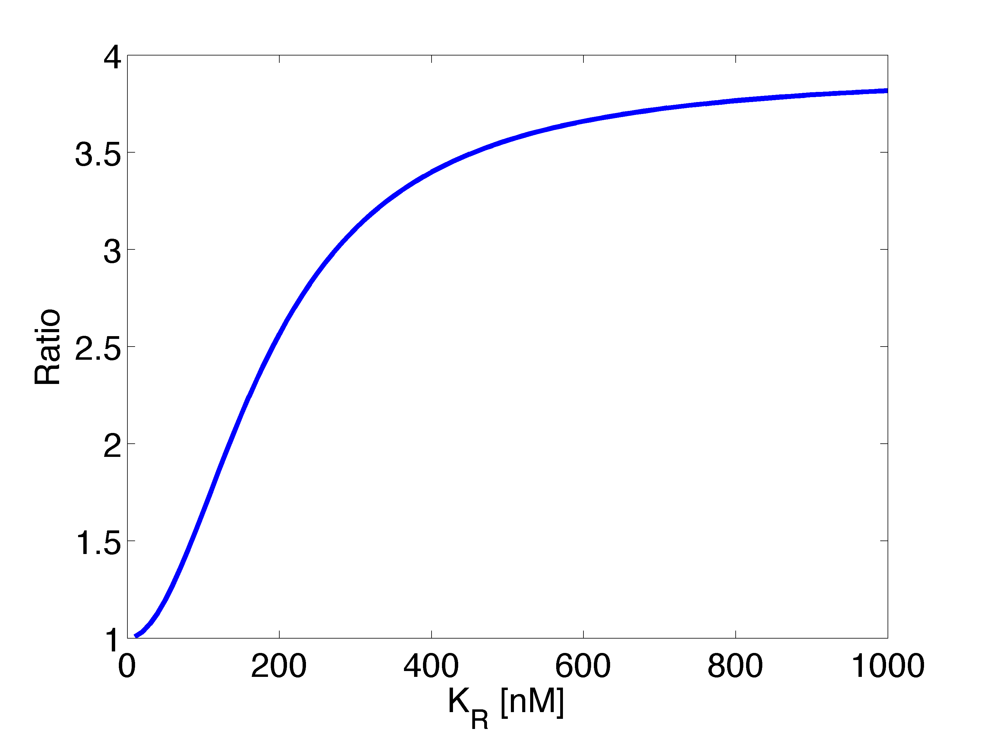
The second protein, $E_{2}$, is responsible to give a colour output that indicate the presence of two mines. Its synthesis should start with some delayed after the first protein, given that the promoter is less sensitive to AHL. However, this protein is also expressed by colonies surrounded by a single mine colony. Our goal is to ensure that the ratio of expression levels for 2 to 1 neighbouring mines is large enough. Taking the limit for this ratio we got:
\begin{align} \lim_{K_{M_{ mut}} \to \infty} \frac{\left(\frac{[AHL_{2}]}{K_{M_{ mut}}}\right)^{2}}{1+\left(\frac{[AHL_{2}]}{K_{M_{ mut}}}\right)^{2}} \Bigg / \frac{\left(\frac{[AHL_{1}]}{K_{M_{ mut}}}\right)^{2}}{1+\left(\frac{[AHL_{1}]}{K_{M_{ mut}}}\right)^{2}} = \lim_{K_{M_{ mut}} \to \infty} \left(\frac{[AHL_{2}]}{[AHL_{1}]} \right)^2 \frac{K_{M_{ mut}}^2 + [AHL_{1}]^2}{K_{M_{ mut}}^2 + [AHL_{2}]^2} = \left(\frac{[AHL_{2}]}{[AHL_{1}]} \right)^2 \end{align}
From the AHL diffusion-reaction model, we learnt that as the number of neighboring mine colonies increases there is a two fold increment on AHL concentration at the receiver colonies; roughly $[AHL_{ 2}] = 2 \cdot [AHL_{ 1}]$. Thus, the best we can hope for is to obtain a ratio of 4.
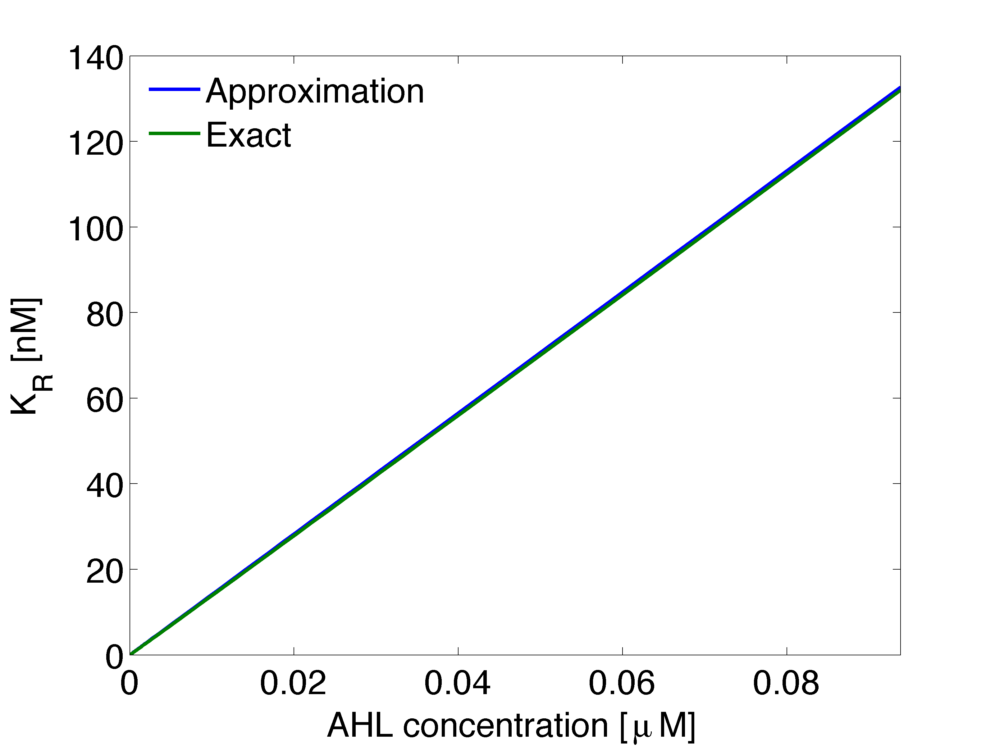
We are still interested in determining the optimal $K_{M_{ mut}}$. For this purpose, we can maximize the difference between the regulation terms for 2 and 1 neighbouring mines:
\begin{align} \operatorname*{max}_{K_{M_{ mut}}} \frac{\left(\frac{[AHL_{ 2}]}{K_{M_{ mut}}}\right)^{2}}{1+\left(\frac{[AHL_{2}]}{K_{M_{ mut}}}\right)^{2}} - \frac{\left(\frac{[AHL_{ 1}]}{K_{M_{ mut}}}\right)^{2}}{1+\left(\frac{[AHL_{ 1}]}{K_{M_{ mut}}}\right)^{2}} \end{align}
Deriving equation 13 w.r.t. $K_{M_{ mut}}$ and set it to zero, we can obtain the following:
\begin{align} \frac{[AHL_{1}]^{2} \cdot K_{M_{ mut}}}{K_{M_{ mut}}^{2} + [AHL_{1}]^{2}} - \frac{[AHL_{2}]^{2} \cdot K_{M_{ mut}}}{K_{M_{ mut}}^{2} + [AHL_{2}]^{2}} = 0 \end{align}
\begin{align} K_{M_{ mut}} = \sqrt[4]{ \frac {[AHL_{1}]^{2} \cdot [AHL_{2}]^{4} - [AHL_{1}]^{4} \cdot [AHL_{2}]^{2} } {[AHL_{2}]^{2}-[AHL_{1}]^{2}} } \end{align}
Once again, considering that $[AHL_{ 2}] = 2 \cdot [AHL_{ 1}]$, we have:
\begin{align} K_{M_{ mut}} = \sqrt{2} \cdot [AHL_{1}] \end{align}
 "
"


